Introduction to CNN
Introduction
This document covers the basic principles of convolutional neural networks (CNN). They are typically used for image classification and segmentation. However, there are other possible applications, such as signal or text processing.
Image filters
The convolutional layer Conv2d is a small filter that slides over an image, transforming it into a new image (of the same or smaller size). Below are the results of four 3x3 filters applied to the top image:

 On the right is an animation of the filter's operation.
The pixels of the original image are shown in blue. The elements of the filter matrix are shown in yellow.
To ensure the resulting image is the same size as the original,
the latter is surrounded by a frame of pixels (gray color), for example, with zero values (this is called padding, details below).
When creating the new image, the filter's numbers are multiplied by the brightness values of the pixels underneath it. All these products are summed, and the result is placed in the first pixel of the new image. Then, the filter shifts to the right, producing the next pixel, and so on.
Here is a numerical example of a filter that highlights vertical edges. Suppose the original image is represented as four cells of a chessboard. We will not surround the image with a frame of zero pixels (padding), so the result of the convolution with a 3x3 filter will be 2 pixels smaller: $$ \begin{vmatrix} 1 & 1 & \color{blue}{\bf 1} & \color{blue}{\bf 1} & \color{blue}{\bf 0} & 0 & 0 & 0\\ 1 & 1 & \color{blue}{\bf 1} & \color{blue}{\bf 1} & \color{blue}{\bf 0} & 0 & 0 & 0\\ 1 & 1 & \color{blue}{\bf 1} & \color{blue}{\bf 1} & \color{blue}{\bf 0} & 0 & 0 & 0\\ 1 & 1 & 1 & 1 & 0 & 0 & 0 & 0\\ 0 & 0 & 0 & 0 & 1 & 1 & 1 & 1\\ 0 & 0 & 0 & 0 & 1 & 1 & 1 & 1\\ 0 & 0 & 0 & 0 & 1 & 1 & 1 & 1\\ 0 & 0 & 0 & 0 & 1 & 1 & 1 & 1\\ \end{vmatrix} ~ \otimes ~ \begin{vmatrix} \color{red}{\bf 1} & \color{red}{\bf 0} & \color{red}{\bf -1} \\ \color{red}{\bf 1} & \color{red}{\bf 0} & \color{red}{\bf -1} \\ \color{red}{\bf 1} & \color{red}{\bf 0} & \color{red}{\bf -1} \\ \end{vmatrix} ~ = ~ \begin{vmatrix} 0 & 0 & \color{green}{\bf +3} & +3 & 0 & 0 \\ 0 & 0 & +3 & +3 & 0 & 0 \\ 0 & 0 & +1 & +1 & 0 & 0 \\ 0 & 0 & -1 & -1 & 0 & 0 \\ 0 & 0 & -3 & -3 & 0 & 0 \\ 0 & 0 & -3 & -3 & 0 & 0 \\ \end{vmatrix} $$ For example, the third pixel in the first row of the resulting image equals (the calculations in each row of the filter are highlighted in parentheses): $(1\cdot 1+1\cdot 0+0\cdot (-1))+(1\cdot 1+1\cdot 0+0\cdot (-1))+(1\cdot 1+1\cdot 0+0\cdot (-1)) = 3$.
 From simple geometric considerations, it is easy to derive the following formula
for the width (and similarly for the height) of the resulting image:
width' = int((width + 2*padding - kernel)/stride + 1),
where padding is the width in pixels of the "fake" frame on the left and right of the image, kernel is the width of the kernel, and stride is the step with which it slides over the image (in the top picture stride=1, padding=0, and in the bottom picture stride=2, padding=1 and in both cases kernel=3).
If stride=1, then to keep the image size unchanged for kernel = 3, 5, 7, ..., you need padding = 1, 2, 3,...
Here is the code in numpy that calculates the convolution (for simplicity without padding and with a stride of one):
h, w, k = 8, 8, 3                      # image height and width, kernel size

img = np.zeros((h, w))                 # image
img[: h//2, : w//2] = 1                # 4 chessboard cells
img[h//2:,  w//2 :] = 1
res = np.empty((h-k+1, w-k+1))         # resulting image

weight = np.array( [ [1,0,-1], [1,0,-1], [1,0,-1] ] )  # edge filter

for i in range(h-k+1):
    for j in range(w-k+1):
        res[i, j] = (weight * img[i: i+k, j: j+k]).sum()
Filter implementation in PyTorch
Let's consider how to compute such filters using the PyTorch library. First, we import the following modules in Python:
import numpy as np
import matplotlib.pyplot as plt
import imageio as imageio
import torch
import torch.nn as nn
We will load an image from a file using the imageio library (which results in a numpy array), convert it from three-channel to single-channel (by averaging over all "color" channels), and display it:
m = imageio.imread("images/yoga.jpg")         # load the image from a file
print(im.shape)                               # (128, 256, 3) = (height, width, channels)
im = im.mean(axis=2)                          # average the "color" channels
print(im.shape)                               # (128, 256)

plt.imshow(im, cmap="gray")                   # display the image
plt.show()
Next, we create an instance of the convolutional layer with one input channel and one output channel (the first two arguments) and a filter (kernel) size of 3x3 (the third argument):
conv = nn.Conv2d(1, 1, kernel_size=3, bias=False, padding=1)
Note the argument bias=False. In general, a bias term is added to the sum of the products of the kernel elements and the pixel intensities of the image (this is a parameter during network training). Here we specify that we do not need a bias term. The padding=1 parameter means that the image is surrounded by a one-pixel-wide frame with zero values (by default). As a result, after applying the convolution, the image size does not change.
Now let's define the filter kernel and place it in the weights of the convolutional layer. Then we will pass the image through it and plot the result:
kernel = [[-1.,-1.,-1.],                      # edge detection filter
          [-1.,+8.,-1.],
          [-1.,-1.,-1.]]

im_tensor = torch.tensor(im.reshape( (1,)+im.shape)).float()

with torch.no_grad():
    conv.weight.copy_( torch.tensor(kernel) ) # set the weights
    im1 = conv(im_tensor)                     # pass the image through the layer

plt.imshow(im1.numpy().reshape(im.shape), cmap="gray")
plt.show()
Since there is no training involved yet, we use the torch.no_grad() context manager to indicate that we do not need to create a computational graph while passing the image through the layer.
Filtering multichannel images
In general, a filter is a 3-dimensional matrix. An image input to the network typically has either one (grayscale) or three (RGB) channels. The output convolutional layer can have an arbitrary number of channels. Below is an example where the layer receives two channels as input and produces three channels as output:

For each output channel, a trainable 3D matrix of parameters (plus bias) is formed. Each of these matrices independently and to the full depth computes the result of the 3D filter's operation.
Thus, when creating a convolutional layer, the key parameters are the number of input channels (filter depth), the number of output channels (number of filters), the kernel size (width and height of the filters), and the stride with which the filter slides over the stack of input images (input channels):
torch.nn.Conv2d(in_channels = 2, out_channels = 3, kernel_size = 2, stride=1,
                padding = 0, padding_mode='zeros', dilation=1)
Technically important parameters are padding and dilation:

If we want the image size to remain unchanged during the convolution, it should be surrounded by a frame of "fake" pixels. For a kernel size of 3, you should set padding = 1, for a kernel size of 5 you should set padding = 2 and so on.
Dilation allows covering a larger area of the image with the same kernel (and consequently the same number of parameters) Despite the "holes," if the filter slides over the image with stride=1, information from all pixels of the input channels will be included in the output channels.
Pooling
 The second key component of convolutional networks is the max pooling layer.
It calculates the maximum pixel value in the input channel within its kernel:
torch.nn.MaxPool2d(kernel_size, stride=None,
                   padding = 0, dilation = 1)
Besides reducing the size of the feature map (width and height of the stack of channels), the MaxPool2d layer also focuses on extracting important features (with the maximum value). Additionally, it makes the network more robust to small shifts in the image (within the MaxPool2d kernel).
Less commonly used is AvgPool2d, which operates similarly to MaxPool2d, but computes the average value of the pixels within the kernel for each channel.
Also noteworthy is AdaptiveAvgPool2d. It is fully equivalent to AvgPool2d, but instead of specifying the kernel size, it accepts the desired output shape. Given the input, it automatically determines the required kernel:
pool = nn.AdaptiveAvgPool2d( (2,3) )
input  = torch.randn(1, 16, 32, 64)
output = pool(input)                    # shape: (1, 16, 2, 3)
Typically, the architecture of a convolutional network consists of a chain of blocks, each composed of Conv2d (creating new features with the filter), ReLU (non-linearity), MaxPool2d (reducing the feature map). Note that the reduction is not necessarily done using the MaxPool2d layer. If the stride of the filter in Conv2d is, for example, 2, then the output images will be 2 times smaller, and if padding is not used, each convolution will "cut off" the perimeter of the map.
Batch normalization
The BatchNorm2d layer is frequently used in convolutional networks (and not only in them). It calculates the mean value mean and standard deviation var for each channel over a data batch $x$ and the output $y$ normalizes them as follows: $$ y = \frac{x-\mathrm{mean}}{\sqrt{\mathrm{var}}}\cdot \mathrm{weight} + \mathrm{bias}. $$ Thus, if the input $x$ has the shape (N,C,H,W), the mean is computed as x.mean((0,2,3)), giving C means for each channel (similarly for var). The trainable parameters weight and bias initially have values of one and zero (for each channel). During training, they are adjusted, allowing the mean of the data propagating through the network to be shifted "appropriately" (bias) and its variance to be scaled (weight).
The calculated mean and var for each batch are averaged using an exponential moving average and stored (but not used in training) are averaged using an exponential moving average and stored (but not used in training):
running_mean = (1−momentum)*running_mean + momentum*mean,
where by default momentum = 0.1.
These averages (as well as the trained coefficients weight, bias)
are used for normalizing data during testing, when we specify model.train(False).
Thus, even if a batch of one example passes through the network during testing,
it will be normalized by this quadruplet, and in the formula above, mean will be replaced by
running_mean, and similarly for var.
Let's output the parameters of the BatchNorm2d layer. Recall that in pytorch, there are three methods to get information about model parameters. The parameters() method is a generator only for trainable parameters (it is passed to the optimizer). The named_parameters() method is a similar generator but also includes parameter names. These two methods also allow access to the gradients of the parameters. Additionally, there is a dictionary state_dict(), which is usually used when saving a model to a file for subsequent loading. It contains only the data and no information about gradients, but there are all parameters, including non-trainable ones (in our case running_mean and running_var):
bn = nn.BatchNorm2d(num_features=3)

for n, p in bn.state_dict().items():
    print(f'{n:20s} : {p.numel()} = {tuple(p.shape)}  {p}')

for n, p in bn.named_parameters():
    print(f"{n:10s} : {p.requires_grad}")
                                 shape   requires_grad   p
    weight               : 3  =  (3,)    True            [1., 1., 1.]
    bias                 : 3  =  (3,)    True            [0., 0., 0.]
    running_mean         : 3  =  (3,)    False           [0., 0., 0.]
    running_var          : 3  =  (3,)    False           [1., 1., 1.]
    num_batches_tracked  : 1  =  ()      False            0
Where to insert batch normalization is a matter of intuition and experimentation. In fully connected networks with asymmetric activation functions (ReLU, Sigmoid) it is worth placing it after them (to eliminate bias). With symmetric functions (Tanh) - before (so that the data is not heavily "cut off" by the activation with a large var).
In convolutional networks, BatchNorm2d is usually inserted immediately after Conv2d, before an asymmetric activation like ReLU. As a result, after ReLU the mean value will be shifted upwards. A similar normalization to a positive mean pixel brightness value is done for input images. Classic values for RGB channels are: mean=(0.485, 0.456, 0.406), std=(0.229, 0.224, 0.225). The considerations are roughly as follows: when using zero-padding, the significant signal needs to be shifted up to reduce the influence of the edges.
VGG
Let's provide an example of a simple, yet quite deep architecture VGG16, that is trained for recognition on colored images of size 224x224 across a thousand classes (cars, cats, and other animals from the ImageNet dataset):
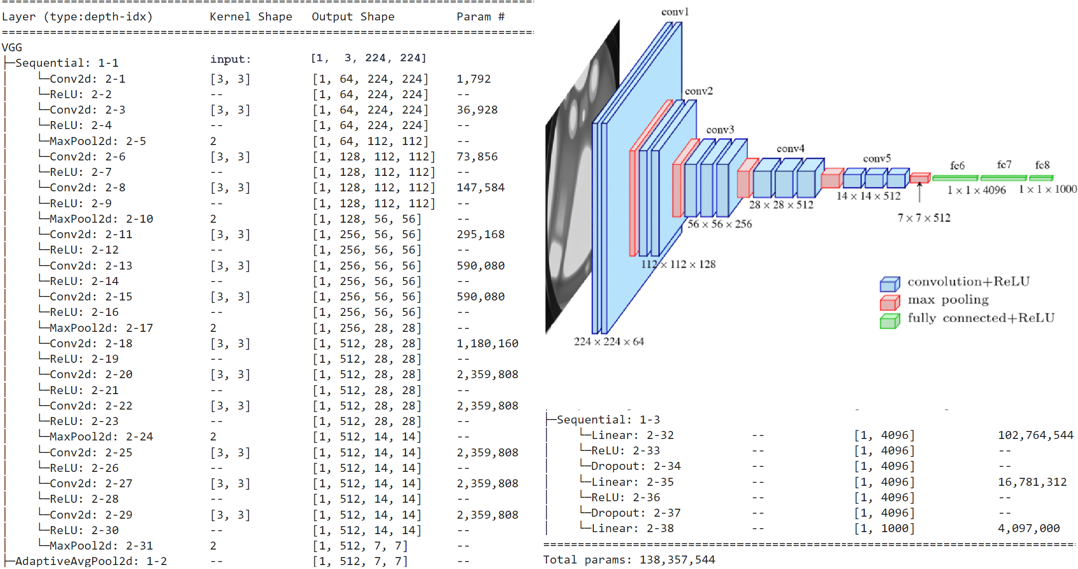
Notice the narrowing and deepening of the feature maps as we move away from the input image. The input to the final fully connected decision network (which contains two additional hidden layers) is a stack of 512 channels of size 7x7. This is a typical property of all CNN architectures (narrowing and deepening).
 A distinctive feature of the VGG architecture is the introduction of several consecutive convolutional layers
with the same kernel without MaxPool2d between them (but, of course, with the ReLU nonlinearity).
This achieves two effects.
First, two consecutive convolutions expand the area of information processed by the filter
(though this is true for all CNNs). For example, two 3x3 convolutions are equivalent in coverage to one 5x5,
convolution but contain fewer parameters. If C is the number of channels, then:
(Cin*3*3+1)*Cout + (Cout*3*3+1)*Cout < (Cin*5*5+1)*Cout
However, if Cin << Cout,
the difference is small. Moreover, the main parameters are primarily learned in the fully connected layers
(see the last column in the VGG architecture above),
so this aspect is not as crucial.
More importantly, there is a nonlinearity ReLU between Conv2d layers. As a result, it is analogous to having two small fully connected layers that deform the feature space more effectively than one larger layer.
ResNet
The ResNet network from Microsoft Labs took first place in the ImageNet competition in 2015. The authors note that deep stacks of convolutional layers lead to significant gradient vanishing, resulting in poor trainability. To solve this problem, they introduced "residual" paths, that make it easier for the gradient to pass through backpropagation. As a result, even networks with 1000 layers can be trained successfully, leading to improved model accuracy.
Let's examine this architecture using the example of the smallest network, ResNet18, from the extensive ResNet network family. The original ResNet18 works with high-resolution images and therefore uses a 7x7 kernel with a stride of 2 and subsequent pooling with a kernel of 3 and a stride of 2 in the first convolutional layer:
ResNet(
  (conv1):   Conv2d(3, 64, kernel_size=(7,7), stride=(2,2), padding=(3,3), bias=False)
  (bn1):     BatchNorm2d(64, eps=1e-05, momentum=0.1, affine=True, track_running_stats=True)
  (relu):    ReLU(inplace=True)
  (maxpool): MaxPool2d(kernel_size=3, stride=2, padding=1, dilation=1, ceil_mode=False)
  ...
As a result, the image size is reduced by 4 times in height and width. For small-resolution images, these layers should be adjusted:
from torchvision import models

model = models.resnet18(pretrained=False, num_classes=10)
model.conv1 = nn.Conv2d(3, 64, kernel_size=(3,3), stride=(1,1), padding=(1,1), bias=False)
model.maxpool = nn.Identity()
Below is the resulting architecture of ResNet18 (with 18 layers, including the input convolution and the classification fully connected layer). It is optimized for input images of size 32x32 pixels (e.g., the CIFAR-10 dataset):

In the blocks where it says 128,/2, the kernel step is stride=2 (with kernel_size=3, padding=1), meaning the width and height of the image are halved. Note that after the feature maps (channels) are reduced in size by half, their number doubles.
The loops on the diagram reflect the structure of the network's two building blocks:
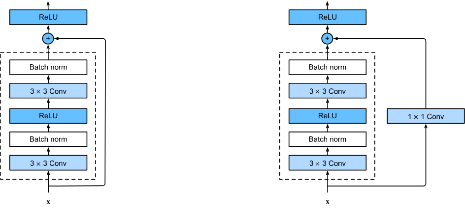
The first corresponds to the solid lines in the architectural diagram. The output of the block, consisting of two convolutions, simply adds (sums) the input value. In the second block (dotted lines in the diagram), the input passes through a convolution with kernel_size=1, stride=1 before mixing. This convolution multiplies the input by trainable weights (and shuffles the channels).
A few important technical points to note:
- All convolutional layers have no bias (bias=False), but BatchNorm2d is used after them.
- There is no pooling layer to reduce the feature maps. Instead, some blocks use stride=2 in the first layer.
Google Inception
Vision transformer (ViT)
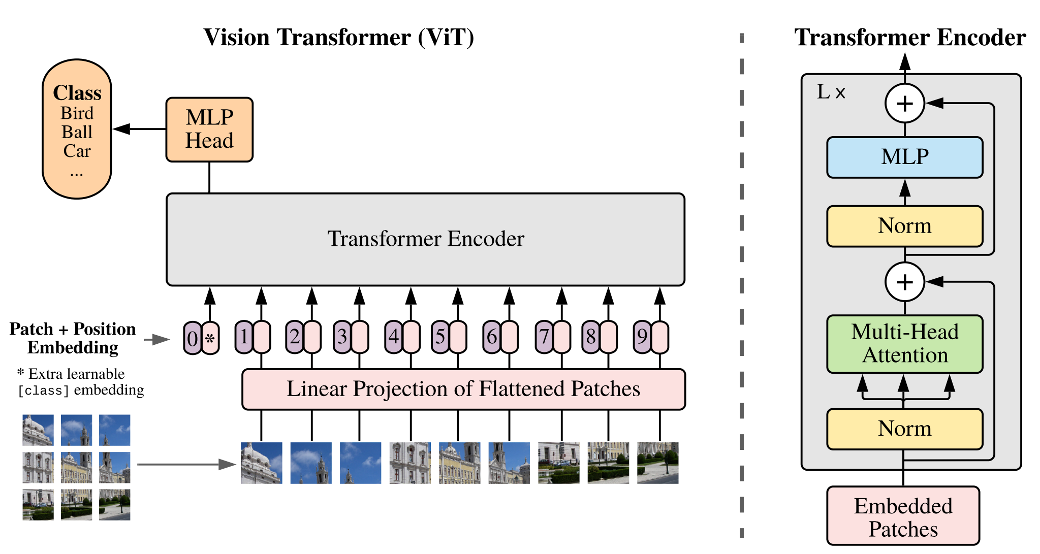
We split an image into fixed-size patches, linearly embed each of them, add position embeddings, and feed the resulting sequence of vectors to a standard Transformer encoder. In order to perform classification, we use the standard approach of adding an extra learnable “classification token” to the sequence.
CLIP
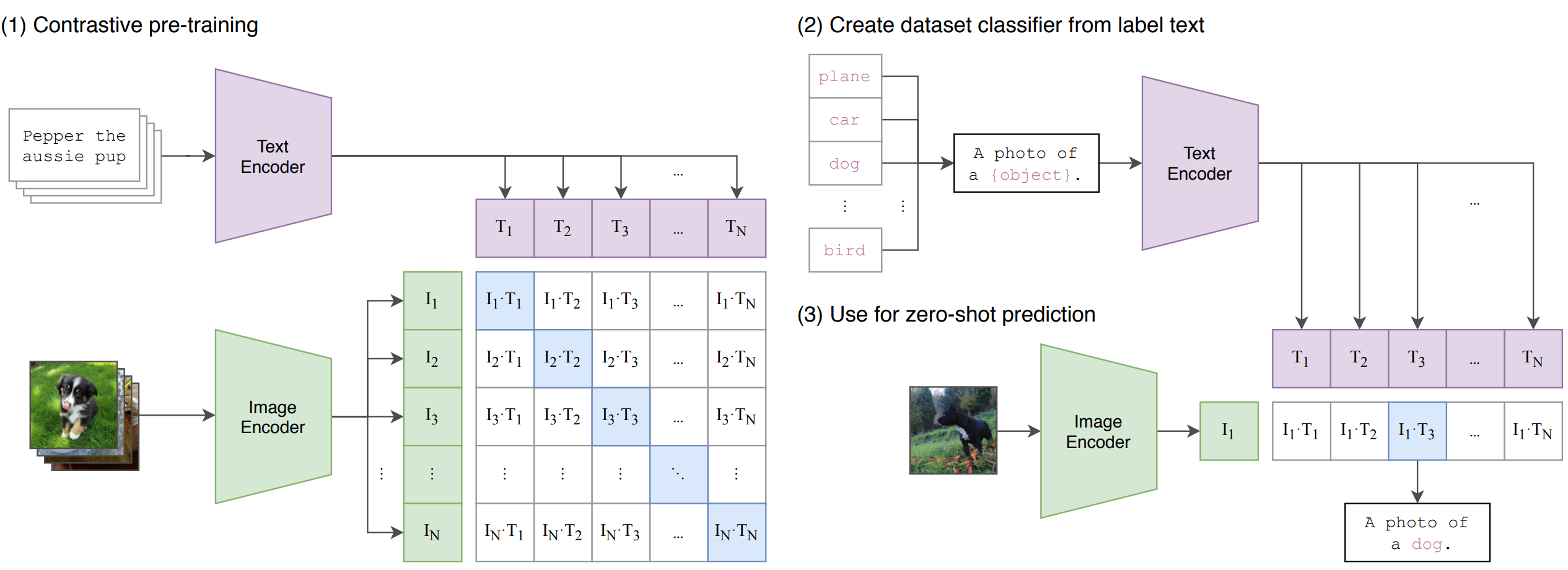
Contrastive Language-Image Pre-training. The batch contains N pairs of image-text, which pass through the ImageEncoder and TextEncoder. We construct a cosine similarity matrix between the vectors of the i-th image and the j-th text. On the diagonal are the correct pairs (image, text) - we maximize these, and minimize the others.
Applications:
- "Generate" text from various n x m templates describing the image (the second picture above).
- There is a new dataset with class names. The names are fed into the TextEncoder, and the given image into the ImageEncoder, and we search for the closest match.
- OpenAI: DALL-E generates images from text. CLIP selects the best 32 out of 512 options, for which the image and text vectors are closest.
Quotes from the article (2021):
- CLIP outperforms the best publicly available ImageNet model while also being more computationally efficient.
- We constructed a new dataset of 400 million (image, text) pairs collected form a variety of publicly available sources on the Internet.
- The resulting dataset has a similar total word count as the WebText dataset used to train GPT-2. We refer to this dataset as WIT for WebImageText.
- We consider two different architectures for the image encoder. For the first, we use ResNet-50, for the second architecture, we experiment with the recently introduced Vision Transformer (ViT)
- For the ResNets we train a ResNet-50, a ResNet-101, and then 3 more which follow EfficientNet-style model scaling and use approximately 4x, 16x, and 64x the compute of a ResNet-50. (RN50x4, RN50x16, and RN50x64).
- For the Vision Transformers we train a ViT-B/32, a ViT-B/16, and a ViT-L/14.
- We train all models for 32 epochs.
- We use the Adam optimizer with decoupled weight decay regularization applied to all weights that are not gains or biases, and decay the learning rate using a cosine schedule.
- We use a very large minibatch size of 32,768.
- The largest ResNet model, RN50x64, took 18 days to train on 592 V100 GPUs while the largest Vision Transformer took 12 days on 256 V100 GPUs.
References
- Kaiming He, et.al - "Deep Residual Learning for Image Recognition" (2015) - ResNet
- Christian Szegedy. et.al - "Rethinking the Inception Architecture for Computer Vision" (2015) Inception
- Alexey Dosovitskiy, et.al - "An Image is Worth 16x16 Words: Transformers for Image Recognition at Scale" (2020) ViT
- Alec Radford et.al - "Learning Transferable Visual Models From Natural Language Supervision" (2021) - CLIP
- Mikhail Konstantinov - "CLIP Neural Network by OpenAI" (habr) - CLIP (ru)
- Mikhail Konstantinov - "Building Neural Networks: Cartoon Animal Classifier. Without Data and in 5 Minutes. CLIP" (colab) - CLIP (ru)
