ML: Binary classification metrics
Introduction
This paper discusses various metrics that characterize the performance of a machine learning model in a binary classification problem. The model, having received the feature vector of an example, assigns it to one of two classes (negative or positive). The names of classes are related to medical diagnosis problems, in which a "good" test result (no disease) is called negative, and a detected disease is called a positive test result. In such problems, the classes are often unbalanced. If we follow the medical analogy, there are fewer examples of positive class in this case than negative class (both in training and test data).
Confusion matrix
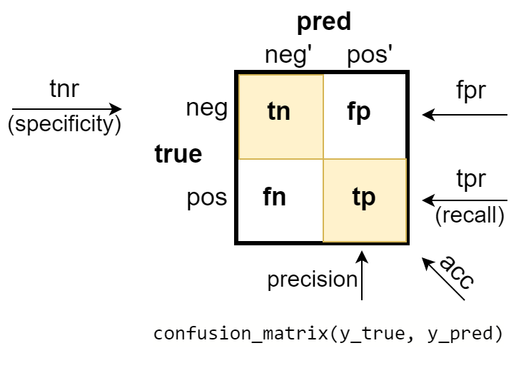
Let the training data contain $\mathrm{neg}$ negative examples and $\mathrm{pos}$ - positive examples. They constitute a set of $N=\mathrm{neg}+\mathrm{pos}$ true examples (training dataset). The number of examples predicted (pred) by the model in the negative (neg') and positive (pos') classes may differ from the true ones. The confusion matrix provides sufficiently complete information about the model's performance. On its diagonal are the numbers of correct predictions:
- true negative (tn) - how many times the model gave a negative class when the example was negative;
- true positive (tp) - how many times the model returned a positive class when the example was positive.
- false negative (fn) - the number of errors when the model produced a negative class, although it was positive;
- false positive (fp) - the number of errors when the model produced a positive class, although it was negative.
The sum of the numbers on the lines corresponds to the number of true negative and positive examples, and their ratio npr (negative-positive-rate) indicates the balance (if npr=1) of classes in the examples:
$$ \mathrm{neg}=\mathrm{tn}+\mathrm{fp},~~~~~~~~~~ \mathrm{pos}=\mathrm{fn}+\mathrm{tp},~~~~~~~~~~ \mathrm{npr} = \frac{\mathrm{neg}}{\mathrm{pos}}. $$Similarly, the sum of the numbers across the columns corresponds to the number of predicted negative and positive examples:
$$ \mathrm{neg}'=\mathrm{tn}+\mathrm{fn},~~~~~~~~~~ \mathrm{pos}'=\mathrm{fp}+\mathrm{tp},~~~~~~~~~~ \mathrm{npr}' = \frac{\mathrm{neg}'}{\mathrm{pos}'}. $$ It is clear that the total number of true and pred examples are equal: $N = \mathrm{neg}+\mathrm{pos}=\mathrm{neg}'+\mathrm{pos}'$. The proportion of negative and positive examples from their total number is equal to: $$ \frac{\mathrm{neg}}{N} = \frac{\mathrm{npr}}{\mathrm{1+npr}},~~~~~~~~~~~~~~~~~~\frac{\mathrm{pos}}{N} = \frac{1}{\mathrm{1+npr}}. $$ In the case of a strong difference in the $\mathrm{npr}$ from unit, in the error function the class examples are usually weighted with rearranged weights (e.g., negative examples with a weight of $1$, and positive - with weight $\mathrm{npr}$).Basic metrics
The main metrics of the model are accuracy (acc) - the accuracy of both classes and the accuracy of each class separately: true negative rate (tnr) or specificity, or selectivity and true positive rate (tpr) or sensitivity, or recall:
$$ \mathrm{acc} = \frac{\mathrm{tn}+\mathrm{tp}}{\mathrm{neg}+\mathrm{pos}},~~~~~~~~~~~ \mathrm{tnr} = \frac{\mathrm{tn}}{\mathrm{neg}},~~~~~~~~~~~~ \mathrm{tpr} = \frac{\mathrm{tp}}{\mathrm{pos}}. $$The accuracy of the positive class tpr is also called completeness. In medical diagnostics, a positive test result is the presence of a disease. Therefore tpr characterizes how complete the model is ("found all the diseases").
Because of this analogy, precision or positive predictive value (PPV) (correct predictions of a pos-class to the number of all predictions of a pos-class) is considered to be accuracy (how accurately a disease is detected): $$ \mathrm{pre} = \frac{\mathrm{tp}}{\mathrm{tp}+\mathrm{fp}} = \frac{\mathrm{tp}}{\mathrm{pos}'}. $$
Sometimes the positive class, according to the subject area, is more important than the negative one, and its examples are much rarer than those of the negative class. In this case, more attention is paid not to $\mathrm{tfr}$ (as the accuracy of the negative class), but to the precision (the accuracy of the positive class). In particular, the balance between completeness and precision is characterized by the metric $F_1$, that is equal to the geometric average between these quantities: $$ \frac{1}{F_1} = \frac{1}{2}\Bigr[\frac{1}{\mathrm{tpr}} + \frac{1}{\mathrm{pre}}\Bigr],~~~~~~~~~~~~~~~F_1 = \frac{2\,\mathrm{tpr}\,\mathrm{pre}}{\mathrm{tpr}+\mathrm{pre}}. $$ The closer $F_1$ to 1 (as well as $\mathrm{tpr}$, $\mathrm{pre}$), the better the model works.
Accuracy and precision are easy to express in terms of relative values:
$$ \mathrm{acc} = \frac{\mathrm{tpr} + \mathrm{tnr}\cdot \mathrm{npr}}{1 + \mathrm{npr}},~~~~~~~~~~~~~~~~~~~ \mathrm{pre} =\frac{\mathrm{tpr}} {\mathrm{tpr}+\mathrm{npr}\cdot(1-\mathrm{tnr})}. $$ If the classes are balanced (npr=1), then the total accuracy is equal to the average accuracy of each class: acc=(tnr+tpr)/2 and regardless of npr, if tnr=tpr, then tnr=tpr=acc.If the classes are noticeably skewed, you can get good accuracy, but the model will be useless (tnr, tpr are in brackets after accuracy):
                     acc  (tnr,   tpr)   pre   npr  npr'
       80 |  0
cm =  --------       0.90 (1.00, 0.50)  1.00    4    9
       10 | 10

       70 | 10
cm =  --------       0.80 (0.86, 0.50)  0.50    4    4
       10 | 10

       60 | 20
cm =  --------       0.75 (0.75, 0.75)  0.43    4    1.9
        5 | 15
ROC - tpr(fpr) curve
Usually, the model does not produce class numbers, but their probabilities or degrees of confidence. In a binary problem with two classes, we can assume that this is a single number equal to $p=0$ for the accuracy of the negative class and $p=1$ - for the accuracy of the positive class. Since $p$ varies in the interval $[0...1]$, to determine the class number, it is necessary to choose the threshold value of the probability $p_0$. If $p \ge p_0$ the example will be assigned to the positive class, and if $p \lt p_0$ - to the negative class. The default value is $p_0=0.5$, however, this is not the only and not always the best option.
For every value $p_0$ there is a confusion matrix and the class accuracy calculated on its basis: $\mathrm{tnr},~\mathrm{tpr}$. Instead of $\mathrm{tnr}$ it is customary to use an additional value to it $\mathrm{fpr}=1-\mathrm{tnr}$. Plot for each $p_0$ on the horizontal axis $\mathrm{fpr}$, and on the vertical axis $\mathrm{tnr}$. The resulting line is called the receiver operating characteristic or ROC-curve:
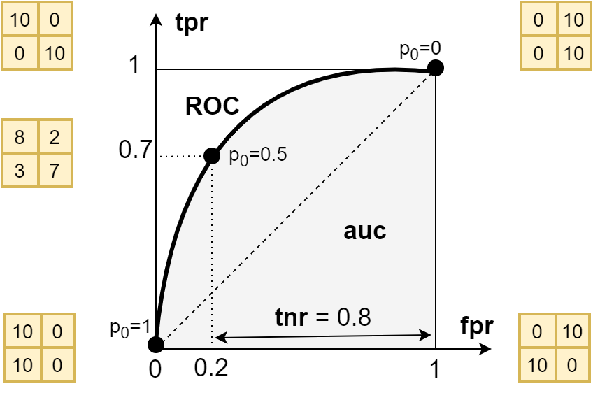
If $p_0=0$ (top right corner), then all examples will belong to the positive class ($\mathrm{fpr}=\mathrm{tpr}=1$), and if $p_0=1$ (bottom, left corner) - to the negative class ($\mathrm{fpr}=\mathrm{tpr}=0$). A good model should tend to the top left corner, (see its confusion matrix). In the example in the figure, at the threshold value of the probability $p_0=0.5$ the accuracy of the negative and positive classes are equal $\mathrm{tnr}=0.8$, $\mathrm{tpr}=0.7$ (the corresponding confusion matrix is shown on the left). By decreasing the threshold, you can increase $\mathrm{tpr}$ by reducing $\mathrm{tnr}$.
AUC metric
The area under the curve is called the auc metric (Area Under Receiver Operating Characteristic). The closer auc is to 1, the better the model is.
Let $n_{0}(p) = N_0(p)/\mathrm{neg}$ - be a share of examples from all $\mathrm{neg}$ examples, belonging to the negative class for which the model gave the probability $p$ (wherein $N_0(p)\,dp$ - is the number of examples of the negative class with probabilities in the interval $[p,\,p+dp]$). Similarly $n_{1}(p) = N_1(p)/\mathrm{pos}$ - is the share of examples of the positive class with probabilities $p$:
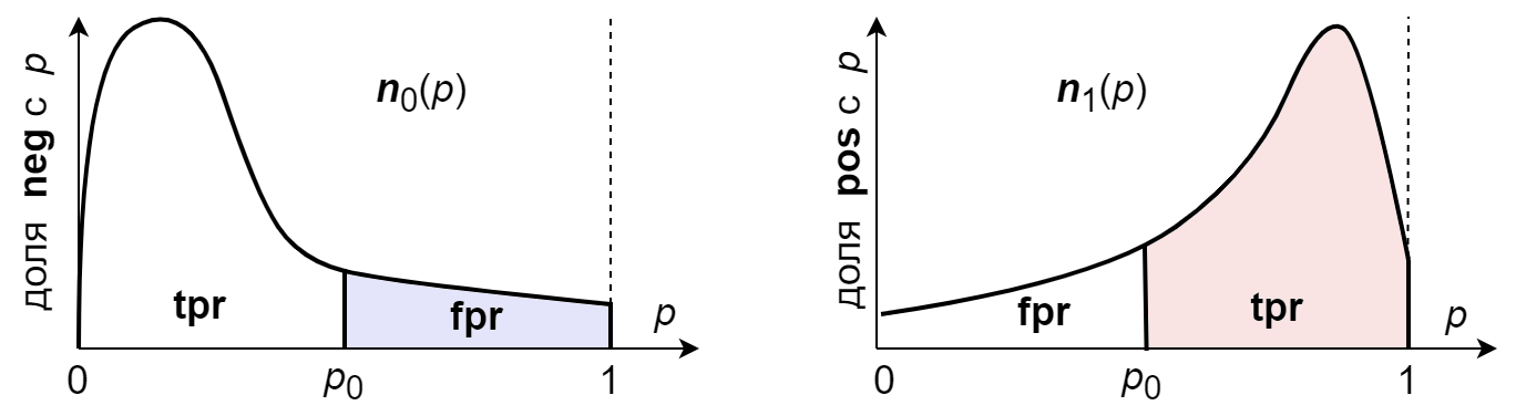
If the curves are the same $n_0(p)=n_1(p)$ (i.e. the prediction does not depend on the class of the example), then $\mathrm{fpr}=\mathrm{tpr}$, which on the ROC diagram corresponds to a dotted line, the area under which is equal to $\mathrm{auc}=1/2$.
If $\mathrm{npr} \gt 1$ - the simplest model will be a prediction for any example of the negative class. In the example below, when $\mathrm{npr} = 4$ such a model will have a fairly high accuracy, but auc will still be 0.5
                     acc  (tnr,   tpr)   pre   npr     auc
       80 |  0
cm =  --------       0.80 (0.80, 0.00)  0.00    4      0.5
       20 |  0
Note that precision is set to 0.0,
even though we have 0/0 by definition. This is due to the fact,
that in calculations we usually add a small number of eps
to eliminate division by zero.
In order to draw an ROC-curve for such an extreme case, we should assume that the probability of the negative class is not strictly zero, but has a narrow peak in the vicinity of zero. Then it follows that tpr=fpt for any $p_0$, i.e. ROC will be straight, and auc=0.5
An example on sklearn
Let's connect libraries and generate a synthetic dataset "two moons" with two classes and two attributes characterizing objects (see figure below):
import numpy  as np
import matplotlib.pyplot as plt

from sklearn.preprocessing  import StandardScaler
from sklearn.utils          import compute_class_weight
from sklearn.metrics        import confusion_matrix, accuracy_score,
from sklearn.metrics        import recall_score, precision_score
from sklearn.datasets       import make_moons

X, Y = make_moons(n_samples=1000, noise=0.2, random_state=42)
Let's calculate the ratio of the number of negative and positive examples (npr), output the matrix forms and the list of classes (np.unique - the list of unique values):
npr = sum(Y==0)/sum(Y==1)
print(X.shape, Y.shape,  np.unique(Y), npr)  # (1000, 2) (1000,)  [0 1] 1.0
Then normalize the data so that their mean equals zero, and the dispersion equals 1. Using the scaler we further normalize the test data with the same parameters:
scaler = StandardScaler().fit(X)    # then use it for testing as well
X = scaler.transform(X)             # (X-X.mean(0)) / X.std(0)
Then, using sklearn, we get the class weights for the logistic regression and perform the actual training:
from sklearn.linear_model import LogisticRegression

w = compute_class_weight(classes=np.unique(Y), y=Y, class_weight ='balanced')

clf = LogisticRegression(C=1, class_weight={0:w[0],1:w[1]})
clf.fit(X,Y)
Probability in logistic regression is a rather conditional concept.
The farther the dot is from the straight line towards the positive class, the closer the "probability" is to 1,
and the farther towards the negative one, the closer to 0.
The value of the predicted classes is calculated with a threshold of 0.5:
probs = clf.predict_proba(X)[:,1] # predict_proba [[P_neg=1-P_pos, P_pos]]
Y_pred = probs > 0.5 # the number of the class
cm = confusion_matrix(Y, Y_pred) # [[435 65]
print(cm) # [ 64 436]]
cm = confusion_matrix(Y, Y_pred, normalize='true')
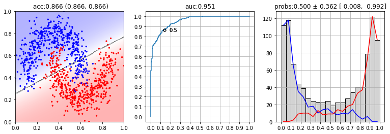
print(f"acc:{accuracy_score(Y,Y_pred):.3f} ({cm[0,0]:.3f},{cm[1,1]:.3f})")
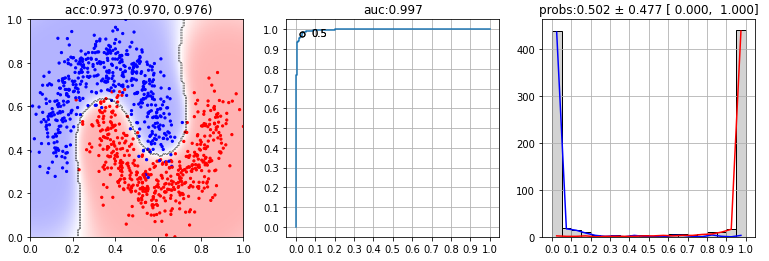
The first diagram below shows all the training examples (red dots are negative, blue ones are positive). The straight line is the class-separating plane obtained by logistic regression. Shading is the confidence level of the model. The second diagram shows the ROC diagram, the value of auc and the dot, that are corresponding to the probability of 0.5 The third diagram shows the probability distribution ($p=0$ - the negative class, $p=1$ - the positive class):
from sklearn.svm import SVC
clf = SVC(probability=True)
The Probabilistic Interpretation of AUC
AUC is equal to the probability that the classifier assigns more weight (probability) to a positive example than to a negative one (ranks a random positive example higher than a random negative one). To prove this important statement, let's calculate the area under the ROC curve (tpr as a function of fpr):
$$ \mathrm{auc} = \int\limits^1_0 \mathrm{tpr}\,d\,\mathrm{fpr} = \int\limits^0_1 \mathrm{tpr}\,\frac{d\,\mathrm{fpr}}{dp}\, dp = -\int\limits^1_0 \mathrm{tpr}\,\frac{d\,\mathrm{fpr}}{dp}\, dp = \int\limits^1_0 \mathrm{tpr}(p)\,n_0(p)\, dp $$ In the third equality, the order of integration has been changed (with a minus sign). Then the definition of $\mathrm{fpr}(p_0)$ is taken into account, as an integral of $n_0(p)$ with $p_0$ at the lower limit. Therefore, its derivative on $p_0$ will give $n_0(p)$ with a minus sign. Then we substitute the definition of $\mathrm{npr}(p_0)$ by $n_1(p)$ and introduce the function $\Delta(x)$ equal to 1, if the logical expression $x$ is true and 0 otherwise: $$ \mathrm{auc} = \int\limits^1_0 \Bigr[ \int\limits^1_{p} n_1(p')\,dp'\Bigr]\,n_0(p)\, dp = \int\limits^1_0\int\limits^1_0 \Delta(p \lt p')~ n_0(p)\,n_1(p')\,\, dp\,dp'. $$The multiplier $n_0(p)\,n_1(p')\,\, dp\,dp'$ means the probability that a randomly chosen negative example has a weight (probability) $p$, and a randomly chosen positive example has the weight $p'$. This multiplier averages $\Delta(p \lt p')$ which gives the average that the order of the weights of the negative and positive examples is correct ($p\lt p'$).
The process of calculating auc by the probabilistic method can be represented as follows. For clarity, we will assume that the probabilities of examples of negative $p^{-}_i$ and positive $p^{+}_j$ classes are sorted in ascending order. In the cell $(i,j)$ of the table put $1$, if $p^{-}_i \lt p^{+}_j$ and 0, if $p^{-}_i \gt p^{+}_j$. If $p^{-}_i = p^{+}_j$, then we will put $0.5$ (we can assume that this is not an exact match, but some identical narrow probability distributions, the correct and incorrect orders for which are equally likely). The sum of the numbers in the cells divided by the "area" $\mathrm{neg}\cdot\mathrm{pos}$ will be equal to $\mathrm{auc}$ (below is the first figure):
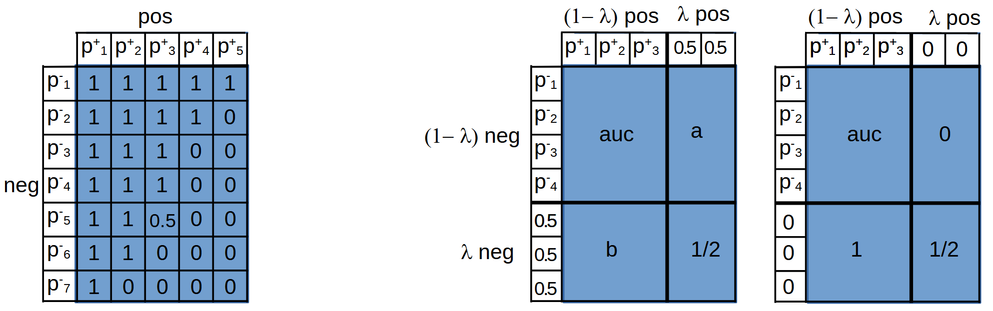
Consider the case where the share $\lambda$ of all examples (both negative and positive) in the test data have properties different from the training data and by some feature we can identify them. Let the model work obviously incorrectly on these "bad" data. What probabilities should be put for bad data to maximize auc? There are two options above: in the first one, all bad data are assigned a probability of $0.5$, and in the second one - the probability of $0$.
If the probability fraction of negative data to the left of $p=0.5$ is greater than $0.5$, then auc between $1-\lambda$ good negative data and bad positive data is equal to $a > 0.5$. Similarly for $b > 0.5$. Therefore, it is better to put the value for the bad data probabilities as $0.5$:
$$ \mathrm{auc}~~ \mapsto~~ (1-\lambda)^2\,\mathrm{auc} + \lambda\,(1-\lambda)\,(a+b) + \lambda^2/2 ~~>~~ (1-\lambda)^2\,\mathrm{auc} + \lambda\,(1-\lambda) + \lambda^2/2 $$Using a probabilistic interpretation of the auc metric, we can write the following function to calculate it:
def auc(y_true, probs):
    x = probs[y_true == 0]                 # negative class probabilities
    y = probs[y_true == 1]                 # positive class probabilities
    z = np.array([np.tile  (x, len(y)),    # x0,x1,...x0,x1,...
                  np.repeat(y, len(x))])   # y0,y0,y0,...,y1,y1,,
    z = z.T                                # [x0,y0], [x0,y1], ..., [xn,ym]

    a = np.zeros_like(z)
    a[z[:,0] <  z[:,1]] = 1.0
    a[z[:,0] == z[:,1]] = 0.5

    return a.mean()
Varia
A loss-function that maximizes auc directly could look like this:
def loss(y_true, y_pred):
    """
    y_true: (N,) - the numbers of classes {0,1}
    y_pred: (N,) - model output for each example (probabilities)
    """
    y_t = torch.cartesian_prod(y_true, y_true)
    y_p = torch.cartesian_prod(y_pred, y_pred)

    L   = (y_t[:,0]-y_t[:,1]) * (y_p[:,1]-y_p[:,0])

    return 0.5 + L.mean()
