Distance and similarity
Introduction
In recognition or clustering tasks, the choice of feature set, which describes an object, plays a key role. If the number of features is $n$, then we speak of an $n$-dimensional feature space. Each object is a point in this space with coordinates $\mathbf{x}=\{x_1,...,x_n\}$. With a successful choice of features, similar (e.g., from a human point of view) objects are usually located close to each other. Accordingly, a certain proximity or distance criterion is necessary.
Metric space
Let the distance $d$ between the points $\mathbf{a}$ and $\mathbf{b}$ in $n$-dimensional space be non-negative, equal to zero for coinciding points (and only for them), and also be symmetric: $$ d(\mathbf{a},\mathbf{b}) \ge 0,~~~~~~~~~~~~d(\mathbf{a},\mathbf{a})=0~~~~~~~~~~~d(\mathbf{a},\mathbf{b})=d(\mathbf{b},\mathbf{a}). $$ In addition, the path (as in Euclidean distance) satisfies the triangle inequality: $$ d(\mathbf{a},\mathbf{b})+d(\mathbf{b},\mathbf{c}) \ge d(\mathbf{a},\mathbf{c}). $$ A space in which the distance between two points satisfies these axioms is called a metric space.
Euclidean distance and normalization
The most popular and familiar distance metric is the Euclidean distance: $$ d(\mathbf{a},\mathbf{b}) = \sqrt{(\mathbf{a}-\mathbf{b})^2} = \sqrt{(a_1-b_1)^2+...+(a_n-b_n)^2} $$ Its use assumes that all components of the feature vector have equal variance, are independent, and are equally important in object classification (i.e., contribute equally to the distance between objects).
Therefore, the mean (center of gravity) of the feature vector and the variance of each feature are calculated (the root of it is called volatility $\sigma_{i}=\sqrt{D_i}$): $$ \bar{\mathbf{x}}\equiv\langle \mathbf{x} \rangle = \frac{1}{N}\sum^N_{\mu=1} \mathbf{x}_\mu,~~~~~~~~~~~~~ \sigma^2_i=D_i = \bigr\langle \bigr(x_i-\bar{x}_i\bigr)^2 \bigr\rangle = \frac{1}{N-1}\sum^N_{\mu=1} \bigr(x_{\mu i}-\bar{x}_i\bigr)^2, $$ where $x_{\mu i}$ is the $i$-th feature of the $\mu$-th object. Then, the feature vectors are normalized. There are different normalization methods: $$ x'_i = \frac{x_i-\mathrm{min}_i}{\mathrm{max}_i-\mathrm{min}_i}, ~~~~~~~~~~~~~~~~~~~~ x'_i = \frac{x_i-\bar{x}_i}{\sigma_i}. $$ The first method is sensitive to individual "outliers", therefore, division by volatility is used more often (the second method). The following normalization is more suitable for neural networks: $$ x'_i = S\Bigr(\frac{x_i-\bar{x}_i}{\sigma_i}\Bigr), $$ where $S(d)=1/(1+\exp(-d))$ is the sigmoid function, which guarantees that the feature will be in the [0...1] range.
Distances between handwritten digits
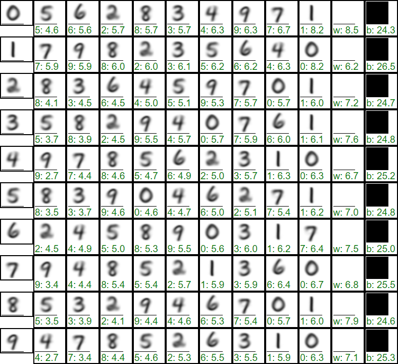
As an example, let's consider the Euclidean distances between handwritten digits represented as grayscale raster images of 28 by 28 pixels. In this case, white color (background) corresponds to a pixel value of zero, and black color corresponds to a value of one. The feature space has 28*28=784 dimensions.
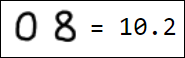
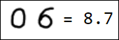
Below are the mean values over 60000 training examples from the MNIST database after skew correction. Each row shows a digit from 0 to 9, and to the right of it, in order of increasing distance, are other digits (Euclidean distance after a colon), as well as the white and black background:
    av   si  min   max
   aver  sigma min   max
0  5.4   1.1   2.1    9.7
1  2.2   1.0   0.6    9.1
2  5.9   0.8   3.5    9.2
3  5.4   0.9   2.5    9.4
4  5.0   0.9   2.6   10.3
5  5.5   0.9   2.8    9.5
6  5.1   1.0   3.0   10.3
7  4.6   1.0   2.4   10.4
8  5.2   1.0   2.9   10.1
9  4.6   1.1   2.5   10.3
The maximum distance in such feature space is 28 (this is the distance between white and black backgrounds). From the distance matrix, it follows that there is a similarity between the numbers (3,5,8) and (4,9,7). The numbers 0 and 1 are the most distinguishable (they are separated by the maximum distance). However, in general, the spread of distances between images is not significant. To the right of the distance matrix, statistics of the distances of individual digits from their mean values in the MNIST database are presented. As can be seen, the digits deviate from the average pattern quite significantly (comparable to distances between patterns of different classes).
Naturally, the set of pixels is not the best option for a feature vector. For example, different writings of the number 1 are quite far from each other in the feature space:
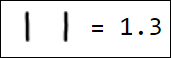 | 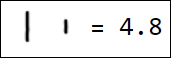 | 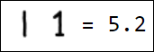 | 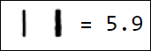 | 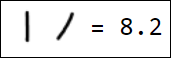 |
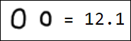 | 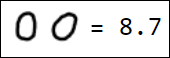 |  |  |  |
Mahalanobis distance
If there is a noticeable difference in the variance or statistical dependence between features, Mahalanobis distance is sometimes used: $$ d^2(\mathbf{a},\mathbf{b}) = \sum_{i,j} \bigr(a_i-b_i\bigr)\, C^{-1}_{ij}\, \bigr(a_j-b_j\bigr), $$ where $C^{-1}_{ij}$ is the matrix inverse of the covariance matrix $C_{ij}=\langle(x_i-\bar{x}_i)(x_j-\bar{x}_j)\rangle$ and curly braces denote averaging over all objects. If the coordinates of the feature vector are not statistically related to each other, then $C^{-1}_{ij}$ is diagonal $\delta_{ij}/D_i$, where $D_i$ is the variance of the feature $x_i$. In this case, the Mahalanobis distance divides the vector components by their variance. This equalizes the significance of their contribution to the total distance.
Note that the Mahalanobis distance is invariant under linear transformations. Indeed, with such a transformation, the covariance matrix changes: $$ x'_i=\sum^n_{k=1}R_{ik}\,x_k~\equiv~ (\mathbf{R}\mathbf{x})_i,~~~~~~~~ C'_{ij}=\langle(x'_i-\bar{x}'_i)(x'_j-\bar{x}'_j)\rangle= \sum_{k,p} R_{ik} R_{jp} C_{kp} = (\mathbf{R}\mathbf{C}\mathbf{R}^T)_{ij}. $$ Therefore: $$ d(\mathbf{a}',\mathbf{b}') = (\mathbf{a}'-\mathbf{b}')^T\mathbf{C}'^{-1}(\mathbf{a}'-\mathbf{b}') =(\mathbf{a}-\mathbf{b})^T\mathbf{R}^T \,(\mathbf{R}\mathbf{C}\mathbf{R}^T)^{-1}\,\mathbf{R}\,(\mathbf{a}-\mathbf{b}) =(\mathbf{a}-\mathbf{b})^T\mathbf{C}\,(\mathbf{a}-\mathbf{b}) =d(\mathbf{a},\mathbf{b}). $$
Instead of using the Mahalanobis distance, it is possible to perform a linear transformation of the feature space once so that $$ \mathbf{x}'=\mathbf{R}\,\mathbf{x}~~~~~~~~~~\mathbf{R}\mathbf{C}\mathbf{R}^T ~=~ \mathbf{1}. $$ As a result of such a transformation, the correlation between features is eliminated, and their variances become equal to one. However, eliminating the correlation between features for all classes is not always reasonable and can worsen their separability.
The Mahalanobis distance can also be used as a measure of proximity to a specific cluster of objects (of a given class), if this cluster has an ellipsoidal shape. In this case, the covariance matrix should be calculated, of course, only for objects included in the cluster.
Other distance functions
Manhattan distance: $$ d(\mathbf{a},\mathbf{b}) = \sum_{i}|a_i-b_i| $$ Maximum distance: $$ d(\mathbf{a},\mathbf{b}) = \mathrm{max} (|a_i-b_i|) $$
Sometimes it's not the absolute position of an object in the feature space that matters, but rather the unit vector pointing from the origin to the object. In this case, the cosine between the vectors can be used as a measure of similarity: $$ d(\mathbf{a},\mathbf{b}) = 1-\frac{\mathbf{a}\mathbf{b}}{|\mathbf{a}|\,|\mathbf{b}|}, $$ where $\mathbf{a}\mathbf{b}=a_1b_1+...+a_nb_n$ is the usual Euclidean dot product of the vectors, and $|\mathbf{a}|$ is the length of the vector.
If all the features are positive and the object vectors are normalized to unit length, then the Kullback-Leibler divergence may be useful: $$ d(\mathbf{a},\mathbf{b}) = \sum^{n}_{i=1} a_{i}\,\ln \frac{a_i}{b_i},~~~~~a_i, b_i \ge 0,~~~~~\sum^n_{i=1} a_i=\sum^n_{i=1} b_i=1. $$ This distance function is not a metric as it is not symmetric and does not satisfy the triangle inequality. However, the Kullback-Leibler divergence is minimized (and equal to zero) when the components of the unit vectors coincide. You can also use its symmetrized version $d(\mathbf{a},\mathbf{b})+d(\mathbf{b},\mathbf{a})$.
Weighted Minkowski distance
Even if the variance of different features is the same, the importance of features for the classification task can be taken into account using weighting coefficients $\omega_i$: $$ d(\mathbf{a},\mathbf{b}) = \Bigr(\sum^n_{i=1} \omega_i\,(a_i-b_i)^p\Bigr)^{1/p} $$ If all $\omega_i=1$ and $p=2$, we return to the Euclidean distance.
Similarity
In addition to distance, the concept of proximity or similarity $s$ is sometimes considered, which satisfies weaker axioms: $$ 0 \le s(\mathbf{a},\mathbf{b}) \le 1,~~~~~~~~~ s(\mathbf{a},\mathbf{a})=1,~~~~~~~~~~~~s(\mathbf{a},\mathbf{b})=s(\mathbf{b},\mathbf{a}). $$ For example, if the components of the feature vector $\mathbf{x}$ take only values 0 or 1 (binary features), then the following similarity functions can be defined: $$ s(\mathbf{a},\mathbf{b}) = \frac{N_{11}(\mathbf{a},\mathbf{b})}{n},~~~~~~~~~~~~~~ s(\mathbf{a},\mathbf{b}) = \frac{N_{11}(\mathbf{a},\mathbf{b})+N_{00}(\mathbf{a},\mathbf{b})}{n},~~~~~~~~~~~~~~ s(\mathbf{a},\mathbf{b}) = \frac{N_{11}(\mathbf{a},\mathbf{b})}{N_{11}(\mathbf{a},\mathbf{b})+N_{10}(\mathbf{a},\mathbf{b}) + N_{01}(\mathbf{a},\mathbf{b})}, $$ where $N_{11}(\mathbf{a},\mathbf{b})$ is the number of matching 1s, $N_{00}(\mathbf{a},\mathbf{b})$ is the number of matching 0s, and $N_{10}(\mathbf{a},\mathbf{b})$ is the number of coordinates equal to 1 in $\mathbf{a}$ and 0 in $\mathbf{b}$ (similarly for $N_{01}$).