ML: Tensors in Numpy
Introduction
Neural network is a function $\mathbf{T}' = F(\mathbf{T})$, that transforms one tensor $\mathbf{T}$ into another $\mathbf{T'}$.Understanding tensors and operations on them is fundamental to understanding how neural networks work.
Tensor is a collection of ordered numbers (elements), indexed by d
integer indices: $\mathrm{t}[i_0,\, i_1,\,...,\, i_{d-1}]$.
The number of indices d is called the tensor dimension.
Each index ranges from 0 to $d_i-1$,
where $d_i$ is called the index dimension.
The listing of the dimensions of all indices: $(d_0,\,d_1,...,d_{d-1})$ is called the tensor shape.
Existing machine learning frameworks handle tensors in a largely similar manner.
Below, we will look at the generic numpy library.
This is not a reference guide for numpy, for that see
scipy.org.
We will focus on the concepts of tensor dimensions and shape,
and how they change with various operations (which is crucial for analyzing neural networks).
Dimension and shape of the tensor
In the numpy library, each tensor t has four basic properties (attributes):
- t.ndim - dimension = the number of indices of the tensor;
- t.shape - shape = a tuple describing the size of each index;
- t.size - the total number of elements in the tensor (if shape=(a,b,c), then size=a*b*c);
- t.dtype - the tensor type (float32, int32,...) is the same for all elements.
If a tensor has one index: t[i] - it is a vector (ndim=1), and if it has two indices: t[i,j] - it is a matrix (ndim=2). Indexes are numbered starting from zero.
The method np.array(lst) converts the list lst (a list of numbers or a list of other lists) into a numpy tensor:
import numpy as np                     #         ndim:    shape:       size:

v = np.array( [ 1, 2, 3] )             # vector:    1     (3,)         3

m = np.array( [ [ 1, 2, 3],
                [ 4, 5, 6] ])          # matrix:    2     (2, 3)       6

t = np.array( [ [[ 1, 2, 3],
                 [ 4, 5, 6]],

                [[ 7, 8, 9],
                 [10,11,12]] ])        # tensor:    3     (2, 2, 3)    12
Note that:
- the shape of a one-dimensional tensor (vector) is (n,) , not (n) , because in Python (n) is a number, not a tuple.
- t = np.array( [[[1]]] ) is a tensor with one number, with shape=(1,1,1) and t.ndim==3, t[0,0,0]==1.
Tensors are usually represented in tabular form: a vector (ndim=1) is a row of numbers, a matrix of shape (rows,cols) is a rectangular table with rows and cols (columns). A three-dimensional tensor (three indices, ndim=3) is represented as a stack of matrices:
It's important not to confuse a vector (n,) with a matrix consisting of one row (1,n) or one column (n,1):
t2  = np.array( [ 1, 2] )             #  shape = (2,)
t12 = np.array( [ [1,2] ] )           #  shape = (1,2)
t21 = np.array( [[1],                 #  shape = (2,1)
                 [2]])


t2[1] == t12[0,1] == t21[1,0] == 2    #  True
Below, matrices with one row or one column are surrounded by a double line to distinguish them from vectors:
$$ \begin{array}{|c|c|} \hline 1 & 2\\ \hline \end{array} ~~~~~~~~~ \begin{array}{|c|} \hline \begin{array}{|c|c|} \hline 1 & 2\\ \hline \end{array} \\ \hline \end{array} ~~~~~~~~~ \begin{array}{|c|} \hline \begin{array}{|c|} \hline 1 \\ \hline 2\\ \hline \end{array} \\ \hline \end{array} $$Sequence of elements
A tensor with the shape = (a,b,c) consists of size = a*b*c
ordered numbers (elements).
The shape of a tensor can be changed (while preserving the number of elements size)
using the reshape method or by directly modifying the shape attribute:
v    = np.array( [1,2,3,4,5,6] )         # shape = (6,)    ndim = 6
m16 = v.reshape( (1,6) )                 # shape = (1,6)   ndim = 6
m32 = v
m23.shape = (2,3)                        # shape = (2,3)   ndim = 6

print(m23)                               #  [ [1,2,3],
                                         #    [4,5,6] ]
$$
\begin{array}{|c|c|c|c|c|c|}
\hline
1 & 2 & 3 & 4 & 5 & 6 \\
\hline
\end{array}
~~~~~~~~\Rightarrow
~~~~~~~~
\begin{array}{|c|}
\hline
\begin{array}{|c|c|c|c|c|c|}
\hline
1 & 2 & 3 & 4 & 5 & 6 \\
\hline
\end{array}\\
\hline
\end{array}
~~~~~~~~\Rightarrow
~~~~~~~~
\begin{array}{|c|c|c|}
\hline
1 & 2 & 3 \\ \hline
4 & 5 & 6 \\ \hline
\end{array}
$$
When changing the shape of a tensor using the reshape method, the result is returned by reference (no new copy of the set of numbers is created). Therefore, if you change the value of an element in m16, it will also change in v:
m16[0,0] = 100
v                                     # [100, 2, 3, 4, 5, 6]
Elements in memory are arranged in ascending index order, starting from the end. For example, for a three-dimensional tensor with the shape (2,1,3) these are 6 numbers in the following order:
t[0,0,0] t[0,0,1], t[0,0,2], t[1,0,0] t[1,0,1], t[1,0,2].
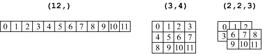
You can change the shape of the tensor in any way, as long as the number of elements remains the same. Below, the arange method creates a vector (one-dimensional tensor) of 12 integers from 0 to 11. Then, references to a matrix and a three-dimensional tensor are obtained. In the latter case, the value -1 in the dimension of the first index asks numpy to independently calculate this dimension (based on the number of elements and the dimensions of the other indices):
v = np.arange(12)                     # [ 0, 1, 2, 3, 4, 5, 6, 7, 8, 9, 10, 11]

m = v.reshape( (3, 4 ) )
t = m.reshape( (-1, 2, 3) )

print(v.shape, m.shape, t.shape)      # (12,) (3, 4) (2, 2, 3)
Tensor axes
Indices are the axes of a tensor. The first index is axis=0, the second is axis=1, and so on. Many methods have an axis parameter. For example, summing along a given axis reduces the number of dimensions ndim by 1.
m = np.ones( (2, 3) )                 # 2x3 matrix of ones:   [ [1,1,1],
                                      #                         [1,1,1]]

print( m.sum(axis=0),                 #  [2. 2. 2.]  sum along rows
       m.sum(axis=1),                 #  [3. 3.]     sum along columns
       m.sum()  )                     #  6.0         sum of all elements
Functions like min, max, mean, median, var, std, argmin, argmax etc. work similarly.
You can slice a subset of elements from a tensor. Below, the first row and the first column are sliced out, and then a 2x2 square matrix is created:
m = np.arange( 6 ).reshape((2,3))     #  [[0, 1, 2],
                                      #   [3, 4, 5]]

v1 = m[0, :]                          #   [0, 1, 2]
v2 = m[0]                             #   same as above (for the first index)
v3 = m[:, 0]                          #   [0, 3]

mm = m[0:2, 0:2]                      # [ [0, 1],
                                      #   [3, 4] ]
Subsets of elements in v1, v2, v3 are obtained by reference rather than by value, so:
v1[0] = 100
m.reshape(-1)                         # [100,   1,   2,   3,   4,   5]
You can change not only the value of a single element but also all elements (below, in the first column):
m[:,0] = -1                           # [[-1,  1,  2],
print(m)                              #  [-1,  4,  5]]
Addition, multiplication and broadcasting
When performing element-wise addition and multiplication of tensors with the same shape, the result retains the same shape: $$ (x+y)_{ijk}:~~x_{ijk}+y_{ijk},~~~~~~~~~~~~~~~~~~ (x*y)_{ijk}:~~x_{ijk}*y_{ijk}. $$ For example (below, np.arange(beg=0, end) generates a vector of integers from beg to end, excluding end):
a = np.arange(3)                      # [0, 1, 2]
b = np.arange(3,6)                    # [3, 4, 5]

a + b                                 # [3, 5, 7]
a * b                                 # [0, 4,10]
Similarly, functions applied to tensors work as: $T'_{ijk}=F(T_{ijk})$. For example: np.exp( ), np.log( ), np.sin( ), np.tanh( ), and a full list can be found at scipy.org.
When adding a vector (n,) or a matrix with one row (1,n) to a matrix (n, m), the rows of the vector or matrix are duplicated, and then addition (or multiplication) of matrices with the same shape occurs. When adding a matrix (n, m) with a matrix of one column (m,1), the columns of the latter matrix are duplicated: $$ \begin{array}{|c|c|} \hline 0 & 1 \\ \hline 2 & 3 \\ \hline \end{array} ~+~ \begin{array}{|c|c|} \hline \mathbf{4} & \mathbf{5} \\ \hline \end{array} ~=~ \begin{array}{|c|c|} \hline 0 & 1 \\ \hline 2 & 3 \\ \hline \end{array} ~+~ \begin{array}{|c|c|} \hline \mathbf{4} & \mathbf{5} \\ \hline \mathbf{4} & \mathbf{5} \\ \hline \end{array}, ~~~~~~~~~~~~~~~~ \begin{array}{|c|c|} \hline 0 & 1 \\ \hline 2 & 3 \\ \hline \end{array} ~+~ \begin{array}{|c|} \hline \begin{array}{|c|} \hline \mathbf{4} \\ \hline \mathbf{5} \\ \hline \end{array} \\ \hline \end{array} ~=~ \begin{array}{|c|c|} \hline 0 & 1 \\ \hline 2 & 3 \\ \hline \end{array} ~+~ \begin{array}{|c|c|} \hline \mathbf{4} & \mathbf{4} \\ \hline \mathbf{5} & \mathbf{5} \\ \hline \end{array} $$
For example:
m = np.array([ [0, 1],
               [2, 3]])

v = np.array(  [4, 5] )

print(m+v)    # [[4, 6],
              #  [6, 8]]
In general, for tensors with different shapes, the broadcasting
algorithm works as follows:- align the number of indices (ndim),by adding ones to the shape of the smaller tensor in front;
- index dimensions are considered compatible if they are equal or one of them is 1;
- increase the dimension of the index with size 1 by duplicating values along that axis:
(3, 1, 4, 1) + (7, 1, 5) = (3, 1, 4, 1) + (1, 7, 1, 5) = (3, 7, 4, 5)For example, adding a matrix with one column and a vector $(3,1) + (2,) = (3,1) + (\underline{1,}2) = (3,2)$: $$ \begin{array}{|c|} \hline \begin{array}{|c|} \hline 1\\ \hline 2\\ \hline 3\\ \hline \end{array} \\ \hline \end{array} ~+~ \begin{array}{|c|c|} \hline 4 & 5 \\ \hline \end{array} ~~ = ~~ \begin{array}{|c|} \hline \begin{array}{|c|} \hline 1\\ \hline 2\\ \hline 3\\ \hline \end{array} \\ \hline \end{array} ~+~ \begin{array}{|c|} \hline \begin{array}{|c|c|} \hline 4 & 5 \\ \hline \end{array} \\ \hline \end{array} ~~ = ~~ \begin{array}{|c|c|} \hline 1 & 1 \\ \hline 2 & 2 \\ \hline 3 & 3 \\ \hline \end{array} ~+~ \begin{array}{|c|c|} \hline 4 & 5 \\ \hline 4 & 5 \\ \hline 4 & 5 \\ \hline \end{array} ~=~ \begin{array}{|c|c|} \hline 5 & 6 \\ \hline 6 & 7 \\ \hline 7 & 8 \\ \hline \end{array} $$
Convolution of vectors and matrices
Key operations include the dot product of vectors and matrix multiplication with convolution: $$ \mathbf{v}\mathbf{u} = \sum^{n-1}_{\alpha=0} v_\alpha\,u_\alpha = u_0\, v_0+...+u_{n-1}\,v_{n-1},~~~~~~~~~~(\mathbf{P}\cdot \mathbf{Q})_{ij} = \sum^{n-1}_{\alpha = 0} P_{i\alpha}\,Q_{\alpha\,j}. $$In numpy both operations are performed using the dot method. For vectors:
u = np.array( [1,2,3] )
v = np.array( [3,2,1] )

print( np.dot(u,v) )             #  10 = 1*3 + 2*2 + 3*1
print( u.dot(v)    )             #  10 - same result
print( np.sum(u*v) )             #  10 - same result
For matrices:
P = np.arange( 6).reshape( (2,3) )
Q = np.arange(12).reshape( (3,4) )

np.dot(P, Q)
P.dot(Q)                         # same result
The table representation of the last multiplication is shown below:

In matrix multiplication, the rows of the first matrix are convolved with the columns of the second matrix.
The figure above shows the calculation of the element
$80$, highlighted in yellow.
To get all the elements, the first row of the first matrix must be convolved with the 4 columns of the second matrix four times.
This gives the first row of the resulting matrix. Then the second row does the same, resulting in the second row of the result.
Convolution of matrices is possible only when the number of columns of the first matrix equals the number of rows of the second matrix.
The following important formula applies for the shapes of the input matrices and the convolution result:
If the first matrix consists of one row and the second consists of one column, their product will still be a matrix, but with one element $(1,\,\underline{2})\cdot(\underline{2},\,1)=(1,\,1)$:
$$ \begin{array}{|c|} \hline \begin{array}{|c|c|} \hline 1 & 2\\ \hline \end{array} \\ \hline \end{array} ~ \cdot ~ \begin{array}{|c|} \hline \begin{array}{|c|} \hline 3\\ \hline 4\\ \hline \end{array} \\ \hline \end{array} ~ = ~ \begin{array}{|c|} \hline \begin{array}{|c|} \hline 11 \\ \hline \end{array} \\ \hline \end{array} $$Convolution by a single index: $(2,\,\underline{1}) \cdot (\underline{1},\,2) = (2,\,2)$ is equal to pairwise multiplication of elements (by the same "row by column" rule): $$ \begin{array}{|c|} \hline \begin{array}{|c|} \hline 1\\ \hline 2\\ \hline \end{array} \\ \hline \end{array} ~ \cdot ~ \begin{array}{|c|} \hline \begin{array}{|c|c|} \hline 3 & 4\\ \hline \end{array} \\ \hline \end{array} ~ = ~ \begin{array}{|c|c|} \hline 3 & 4 \\ \hline 6 & 8 \\ \hline \end{array} = c_{i1}r_{1j} $$
Transpose of a matrix
The transposition operation rearranges elements such that rows and columns are swapped. If the shape of the original matrix was $(n,\,m)$, the transposed matrix will have the shape $(m,\,n)$:
$$ t^T_{ij} = t_{ji},~~~~~~~~~~~~~~~~~~~ \mathrm{transpose}~~ \begin{array}{|c|c|c|} \hline 0 & 1 & 2 \\ \hline 3 & 4 & 5 \\ \hline \end{array} ~ = ~ \begin{array}{|c|c|c|} \hline 0 & 3 \\ \hline 1 & 4 \\ \hline 2 & 5 \\ \hline \end{array} $$In numpy, transposition is performed using the transpose() method or the .T attribute:
a = np.arange(6).reshape(2,3)
b = a.T
b.shape                        # (3, 2)
It is important to note that transposition and reshaping dimensions using reshape lead to different orders of elements:
v = np.arange(6)
m = v.reshape(3,2)

m1 = m.reshape(2,3)            # m1 = [[0 1 2]      m2 = [[0 2 4]
m2 = m.T                       #       [3 4 5]]           [1 3 5]]
Transposition does not create a new matrix (it returns a reference, not the values). Therefore:
m2[0,0]=100
m                              #  [ [100, 1, 2],
                               #    [  3, 4, 5]]
A non-square matrix can be multiplied by itself only after transposing it (otherwise, the rule of matching the number of columns and rows will not be satisfied):
a = np.arange(6).reshape(2,3)

np.dot(a, a.T)      # [ [ 5, 14],  [14, 50] ]                         (2,3)(3,2)=(2,2)
np.dot(a.T, a)      # [ [ 9, 12, 15], [12, 17, 22], [15, 22, 29]]     (3,2)(2,3)=(3,3)
For tensors of arbitrary dimensionality, the transposition operation rearranges all indices in reverse order $t^T_{ijk...}=t_{...kji}$:
x = np.empty( (4,3,2,7) )   # array with "garbage" element values

print(x.T.shape)            # (7,2,3,4)
As with matrices, such index rearrangement results in a different order of elements compared to simply changing the shape attribute.
Tensor multiplication with convolution
For arbitrary tensors, the dot convolution operation works on the principle of last index with second-to-last: $$ (\mathbf{a}\,.\mathbf{b})_{ijkm} = \sum_\alpha a_{ij\underline{\alpha}}\,b_{k\underline{\alpha} m}. $$
The multiplication of a vector $\mathbf{V}$ and a tensor $\mathbf{T}$, regardless of the tensor's
ndim, is interpreted as follows.
The tensor's last two indices are taken, and convolutions are performed
(the second case follows the principle of "last with second-to-last"):
If the tensor has ndim=2 (a matrix), then the vector on the right becomes a column, and on the left, it becomes a row:
$$ \begin{array}{|c|c|} \hline 1 & 1 \\ \hline \end{array} \cdot \begin{array}{|c|c|c|} \hline 1 & 1 & 1\\ \hline 1 & 1 & 1\\ \hline \end{array} \cdot \begin{array}{|c|c|c|} \hline 1 \\ \hline 1 \\ \hline 1 \\ \hline \end{array} ~=~ 6 $$ In this case, the shapes follow the rule: $\underline{(2,)\,. (2,3)}\,. (3,) = (3,)\,. (3,) = $ scalar or $(2,)\,. \underline{(2,3)\,. (3,)} = (2,)\,. (2,) = $ the same scalar.Other convolution operations
There is another method of convolution called matmul (with the @ operator for it). For ndim = 2, the result of this convolution is the same as the dot convolution. The differences start when ndim > 2.
In this case, tensors are interpreted as stacks of 2D
matrices by the last two indices.
These 2D matrices are multiplied independently in each "plane of the stack".
The last two indices of the tensors are fixed, and the tensors are broadcasted over the remaining indices.
For vectors, an index is added and then removed.
$$
(\overline{1,}\, 2, 3) ~@~ (\overline{3, 2,} \,3, 5) ~~~\Rightarrow~~~
(\overline{1,1,}\, 2, 3) ~@~ (\overline{3, 2,}\,3, 5) ~~~\Rightarrow~~~
(3, 2, 2, \underline{3}) ~@~ (3, 2, \underline{3}, 5) ~~~\Rightarrow~~~ (3, 2, 2, 5)
$$
Multiplying $(\mathbf{3},~2,~3)~ @ ~(\mathbf{3,~2},~3,~5)$ is not possible
because they cannot be broadcasted over the "bold" indices
(matrix multiplication must occur over the last two indices and they remain unchanged).
As in dot, the size of the last index of the first tensor and the second-to-last index of the second tensor must match.
The universal convolution np.tensordot(A, B, axes = (axes_A, axes_B)) performs a convolution along the specified indices of tensors A and B:
A = np.empty( (3,4,5) )
B = np.empty( (1,3,4,2) )

C = np.tensordot(A,B, axes=([0,1], [1,2]))  # 0th with 1st and 1st with 2nd
C.shape                                     # (5, 1, 2)
If axes = 1, then it is the standard dot product. If axes = 0, then it is the direct product $A\otimes B$.
Element initialization
The initialization of tensor elements can be very diverse. For the following methods, the elements will have the type float64:
y = np.empty( (2,3) )                 # 2 rows and 3 columns without initialization

x = np.zeros( (2,3) )                 # 2 rows and 3 columns of zeros

x = np.ones ( (2,3) )                 # 2 rows and 3 columns of ones
x = np.eye(3)                         # 3x3 identity matrix

x = np.linspace(0, 1, 3)              # [0. , 0.5, 1. ]  (x=beg,  x <= end, num)
The following functions result in integer elements of type int32:
x = np.arange(3)                      # [0, 1, 2] from 0   to end - 1
x = np.arange(1,3)                    # [1, 2]    from beg to end - 1
x = np.arange(10, 30, 5)              # [10, 15, 20, 25] (i=beg,  i < end, i+=step)
The element type of these tensors depends on the initialization method arguments:
x = np.empty_like(y)                  # same shape as y, but with random values
x = np.zeros_like(y)                  # zeros with the same shape as tensor y

x = np.full((2,3), 5)                 # 2x3 filled with fives (5 is int32; 5. is float64)
x = np.tile(y, (2, 2))                # tile tensor y into a 2x2 matrix
The element type can be changed during initialization:
x = np.ones  ((4,), dtype=np.int64)
x = np.arange(3,    dtype=np.float32)
Random tensors
Random single numbers:x = np.random.seed(1) # fix the random seed x = np.random.randint(0,10) # one uniformly distributed integer from [0...10) int32 x = np.random.uniform(0,10) # one uniformly distributed number from [0...10) float64 x = np.random.normal (0, 1) # one Gaussian random number with aver=0, sigma=1 float64Random tensors of type float64:
x = np.random.random ( (2,3) )        # 2x3 uniformly distributed random numbers [0...1)
x = np.random.normal (0, 1, (10,) )   # 10 Gaussian random numbers with aver=0, sigma=1
Random tensors of type int32:
x = np.random.randint(0, 4, (10,) )   # 10 uniformly distributed integers [0...3]
x = np.random.permutation(5)          # a permutation of the sequence 0,1,..,4
Generating integers from 0 to len(prob)-1 with probabilities prob:
prob=[0.1, 0.1, 0.3, 0.25, 0.25]
np.random.choice(len(prob), 3, p=prob)# [2, 2, 4] : 3 random numbers with given prob
Useful extras
To select elements that meet a condition:
a = np.array([0,2,4,6,8])

idx = a >  2                      # [False, False,  True,  True,  True]
b   = a[idx]                      # [4, 6, 8]
Another option: numpy.where(condition, x[, y]) - from x or y:
a = np.arange(10)                 # [0, 1, 2, 3, 4, 5, 6, 7, 8, 9]
np.where(a < 5, a, 10*a)          # [0, 1, 2, 3, 4, 50,60,70,80,90]
To shuffle elements of two arrays synchronously:
a = np.array([0,2,4,6,8])
b = np.array([1,3,5,7,9])

idx = np.random.permutation(a.shape[0])   # integer indices in random order
a = a[idx]                                # [0 8 4 6 2]
b = b[idx]                                # [1 9 5 7 3]
To append arrays to each other, you need to define the shape with a zero first index for the initial empty array (not necessary for one-dimensional arrays)
ar1 = np.array([], dtype=np.float32).reshape(0,2)  # (0,2)

ar1 = np.vstack([ar1, np.zeros((1,2))])            # (1,2)
ar1 = np.vstack([ar1, np.ones ((3,2))])            # (4,2)
...
If the final size is known, it's better to allocate it immediately and change values.
The number of significant digits and other properties of tensor output can be set with the method:
np.set_printoptions(precision=3, suppress=True) # 3 digits after the decimal point in print
