ML: Combinatorics and Probability
Introduction
When calculating the probabilities of elementary events, it is often necessary to count the number of possible outcomes. This task falls under the domain of combinatorics. It's a rather unique branch of mathematics. The problems it addresses may seem quite complex until their solutions are presented. Immediately after that, they appear to be absolutely elementary. This document continues the introduction to probability theory and is dedicated to the elements of combinatorics and some important probability distributions.
Permutations
 The number of possible permutations of $n$ numbered objects is equal to the
factorial of the number of objects:
$$
n!=n\cdot(n-1)\cdot....\cdot 1.
$$
Indeed, the first object (balls on the right) can be placed
in one of $n$ positions. For each of these possibilities, the second object can be placed
in one of the $n-1$ remaining free positions.
This can be done in $n\cdot(n-1)$ ways. For each of these, the third object is left with $n-2$ positions,
and so on.
The number of possible permutations of $n$ numbered objects is equal to the
factorial of the number of objects:
$$
n!=n\cdot(n-1)\cdot....\cdot 1.
$$
Indeed, the first object (balls on the right) can be placed
in one of $n$ positions. For each of these possibilities, the second object can be placed
in one of the $n-1$ remaining free positions.
This can be done in $n\cdot(n-1)$ ways. For each of these, the third object is left with $n-2$ positions,
and so on.
It's convenient to define that $0!=1!=1$. For large values of $n$, the factorial $n!$ grows very rapidly, and the approximate Stirling's formula is valid: $$ \ln n! \approx n\ln n - n + \ln\sqrt{2\pi n} + \frac{1}{12 n}, $$ which works well even for small $n$. For example, $\ln 5! = 4.78749$, and Stirling's formula yields $4.7875\underline{1}$.
◊ How many ways are there to seat $n$ people at a table?
The number of permutations of people is equal to $n!$. It doesn't matter whether they sit along
a rectangular table or around a circular one.
Arrangements
 Let there be $n$ numbered balls in a closed urn.
Randomly, $m \le n$ balls are drawn from the urn sequentially (without replacement).
Let's find the number of different outcomes of this procedure.
The first ball drawn can be any of the numbered balls $1,...,n$. For each of them,
the second ball can be one of the remaining $n-1$ balls, and so on.
This quantity is called the arrangements $m$ from $n$:
$$
A^m_n = n\cdot (n-1)\cdot\,...\cdot (n-m+1) = \frac{n!}{(n-m)!},
$$
where the product is multiplied and divided by $(n-m)!$. In the figure on the right $n=3$, $m=2$ and $A^2_3=6$.
Note that the outcomes of the draws can be represented as $A^m_n$ distinct $m$-tuples
of non-repeating integers
$(x_1,...,x_m)$, where $x_i\neq x_j$, and the values lie in the range $1\le x_i\le n$.
Let there be $n$ numbered balls in a closed urn.
Randomly, $m \le n$ balls are drawn from the urn sequentially (without replacement).
Let's find the number of different outcomes of this procedure.
The first ball drawn can be any of the numbered balls $1,...,n$. For each of them,
the second ball can be one of the remaining $n-1$ balls, and so on.
This quantity is called the arrangements $m$ from $n$:
$$
A^m_n = n\cdot (n-1)\cdot\,...\cdot (n-m+1) = \frac{n!}{(n-m)!},
$$
where the product is multiplied and divided by $(n-m)!$. In the figure on the right $n=3$, $m=2$ and $A^2_3=6$.
Note that the outcomes of the draws can be represented as $A^m_n$ distinct $m$-tuples
of non-repeating integers
$(x_1,...,x_m)$, where $x_i\neq x_j$, and the values lie in the range $1\le x_i\le n$.
Combinations
 Let there be $n$ numbered balls in an urn. We draw (without replacement) $m$ balls, without considering their order.
For clarity, let's assume that at the end, the balls are ordered by increasing number:
$(x_1 \lt x_2 \lt ....\lt x_m)$, where $1 \le x_1\le n$.
The number of such $m$-tuples is called the combinations of $m$ from $n$.
Let there be $n$ numbered balls in an urn. We draw (without replacement) $m$ balls, without considering their order.
For clarity, let's assume that at the end, the balls are ordered by increasing number:
$(x_1 \lt x_2 \lt ....\lt x_m)$, where $1 \le x_1\le n$.
The number of such $m$-tuples is called the combinations of $m$ from $n$.
Since $m$ numbered objects can be arranged in $m!$ ways, the values of $A^m_n$ must now be reduced by a factor of $m!$ (since all their permutations are not significant). As a result, we obtain binomial coefficients: $$ C^m_n = \frac{n!}{m!\,(n-m)!}. $$ It's easy to see that $C^n_n=1$ (we simply drew all the balls), and $C^1_n=n$ (we drew one out of $n$ balls).
The Binomial Theorem is a generating function for $C^m_n$ (the coefficients of its expansion in a series with respect to $x$ give $C^m_n$): $$ (1+x)^n ~=~ 1 +\frac{n}{1!}\,x+\frac{n\,(n-1)}{2!}\,x^2 +...+ x^n ~=~\sum^n_{m=0} C^m_n\, x^m. $$ Here are also a few useful identities: $$ C^m_n=C^{n-m}_n,~~~~~~~~~~~~C^{m+1}_{\,n\,+1} - C^{m+1}_{\,n} = C^m_n,~~~~~~~~~~~~~ \sum^n_{m=0} C^m_n = 2^n,~~~~~~~~~~~~~ \sum^n_{m=0} (C^m_n)^2 = C^n_{2n}. $$ The first two follow from the definition, and the last one follows from the generating function.
◊ How many sequences of zeros and units of length $n$ exist with exactly $m$ units?
There are $C^m_n$ such sequences. For example, for $n=4$, $m=2$, $C^2_4=6$ they are: $1100$, $1010$, $1001$, $0110$, $0101$, $0011$.
Indeed, let's make the units distinguishable (number them). The first unit can be placed in any of the $n$ positions.
The second one, in any of the remaining $n-1$ positions, and so on, i.e., a total of $~~~n\cdot (n-1)\cdot...\cdot (n+m-1)$ ways,
which should be divided by $m!$ (the units are indistinguishable - all their permutations are equivalent).
Another reasoning is possible as well. Consider some sequence (e.g., $1100$).
All its variations are $n!$ permutations of $n$ digits, among which $m!$ permutations of $m$ units
and $(n-m)!$ permutations of $n-m$ zeros are indistinguishable. Therefore, we have $n!/m!(n-m)!=C^m_n$ variants.
Binary sequences
arise in the binomial distribution and in the derivation of the Fermi distribution
(arrangements of $m$ fermions among $n$ states, which cannot have the same state).
Compositions
 ✒ A useful relationship is the number of possible decompositions (compositions)
of the number $n$ into $k$ summands: $n_1+...+n_k = n$. Let $n_i \gt 0$.
Let's represent the number $n$ as $n$ units separated by empty spaces: $1\square 1\square 1$.
On these $n-1$ spaces, there should be $k-1$ commas separating the summands, and in the remaining ones,
there should be plus signs forming these summands. For example, $3 = 1+2$ is represented as $1\,,\,1+1$. Since the commas are indistinguishable,
the number of combinations
(ways of arrangement) of commas is equal to $C^{k-1}_{n-1}$. If some of the $k$ summands $n_i$ can be zeros, then the sum should be rewritten as follows:
$(\tilde{n}_1-1)+...+(\tilde{n}_k-1)=n$ or $\tilde{n}_1+...+\tilde{n}_k=n+k$, where all $\tilde{n}_i \gt 0 $.
Thus:
$$
\text{The number of compositions}~~~~
n_1+...+n_k = n~~~\text{equals}~~~~~~~~~
\left\{
\begin{array}{lll}
C^{k-1}_{n-1}, & if & n_i \gt 0\\
C^{k-1}_{n+k-1},& if & n_i \ge 0\\
\end{array}
\right..
$$
✒ A useful relationship is the number of possible decompositions (compositions)
of the number $n$ into $k$ summands: $n_1+...+n_k = n$. Let $n_i \gt 0$.
Let's represent the number $n$ as $n$ units separated by empty spaces: $1\square 1\square 1$.
On these $n-1$ spaces, there should be $k-1$ commas separating the summands, and in the remaining ones,
there should be plus signs forming these summands. For example, $3 = 1+2$ is represented as $1\,,\,1+1$. Since the commas are indistinguishable,
the number of combinations
(ways of arrangement) of commas is equal to $C^{k-1}_{n-1}$. If some of the $k$ summands $n_i$ can be zeros, then the sum should be rewritten as follows:
$(\tilde{n}_1-1)+...+(\tilde{n}_k-1)=n$ or $\tilde{n}_1+...+\tilde{n}_k=n+k$, where all $\tilde{n}_i \gt 0 $.
Thus:
$$
\text{The number of compositions}~~~~
n_1+...+n_k = n~~~\text{equals}~~~~~~~~~
\left\{
\begin{array}{lll}
C^{k-1}_{n-1}, & if & n_i \gt 0\\
C^{k-1}_{n+k-1},& if & n_i \ge 0\\
\end{array}
\right..
$$
◊ How many ways are there to distribute $m$ indistinguishable balls into $n$ numbered boxes?
Let's denote by $N_i$ the number of balls in the $i$-th box. Then $N_1+...+N_n=m$, where $N_i\ge 0$ (there may be no balls in the box).
Therefore, the number of placement options is $C^{n-1}_{m+n-1}$.
This problem lies at the heart of the derivation of the quantum Bose-Einstein distribution
(arrangement of $m$ identical bosons in $n$ states).
◊ Suppose midterms last for $d$ days and consists of $x$ exams. According to the rules,
there should be at least one day off after an exam. What is the probability
that some exam will fall on the first day of the session (assuming a random scheduling)?
Let's add one day to the session, which will always be a day off. Pairs of days ($x$ in total) for exams plus a day off: $(e,o)$ will be placed
inside the session, dividing them by $d_i\ge 0$ days: $d_1(e,o)d_2(e,o)d_3....(e,o)d_k,~$ where
$k=x+1$ и $d_1+...+d_k=n=d+1-2\,x$. Since $d_i\ge 0$,
the number of possible schedules is $N = C^{k-1}_{n+k-1}\cdot x! = A^{x}_{d+1-x}$.
Similarly, the number of schedules
with an exam on the first day is calculated : $(e,o)d_1(e,o)d_2....(e,o)d_k$. Now $k=x$ and $N_1 = C^{x-1}_{d-x}\cdot x! = x\, A^{x-1}_{d-x}$.
Therefore, the required probability is $P=N_1/N = x \, A^{x-1}_{d-x}/A^{x}_{d-x+1} = x/(d-x+1).$

Sampling with replacement
We will draw $m$ balls from the urn, assuming that the number of the ball is recorded, after which it is returned to the urn. Unlike sampling without replacement, the numbers in the list can be repeated. If we keep track of the order of the drawn balls, each combination is a number with $m$ digits in the base-$n$ numeral system: $(x_1x_2...x_m)$, where $n$ is the number of balls in the urn. The number of such numbers is equal to $n^m$. Indeed, there can be $n$ "digits" in the first digit. For each such possibility there can again be $n$ "digits" in the second digit, and so on: $n\cdot n\cdot ...$ (repeated $m$ times). One can also envision a tree with $n$ branches emanating from the root (the first "digit"), from each branch $n$ branches again emanate (the second "digit"), and so on.
The situation gets more complicated when the order of the drawn balls is not tracked, as they are shuffled and ordered at the end. Therefore, it is necessary to find the number of all possible $m$-tuples of the form $(x_1\le x_2 \le ...\le x_m)$, where $1 \le x_i \le n$. Dividing $n^m$ by $m!$ is not possible, as in the situation with combinations, because the sequences may contain repeated numbers (instead of $\lt$ we have $\le$).
 Let's denote the number of desired combinations as $(m,n)$.
Obviously $(1,n)=n$. Let's prove by induction that
$$
(m,n) = C^m_{n+m-1}.
$$
Let's find the number of $(m+1,n)$ sequences $(x_1\le ...\le x_{m+1})$.
For $x_1=1$, there will be $(m,n)$ options for $(x_2\le ...\le x_{m+1})$.
The number of sequences with $x_1=2$ is $(m,n-1)$, since the numbers in the list
$(x_1\le ...\le x_{m+1})$, $2\le x_i\le n$ can be
decreased by $1$, resulting in $1\le x_i\le n-1$.
Similarly, continue to $(m,1)$ when $x_1=n$:
$$
(m+1,n) ~=~ (m,1)+\sum^n_{k=2} (m,k) ~=~ C^{m}_{m}+\sum^n_{k=2} C^m_{k+m-1} ~=~
C^{m}_{m} + \sum^n_{k=2} (C^{m+1}_{k+m}-C^{m+1}_{k+m-1}) = C^{m}_{m} - C^{m+1}_{m+1}+ C^{m+1}_{n+1},
$$
where in the second equality, we substitute $(m,n) = C^m_{n+m-1}$, and in the third one
we take into account the second identity for binomial coefficients.
In the obtained sum of differences all terms cancel out except for the first and last parts. Since $C^m_m = C^{m+1}_{m+1}$,
we get $C^{m+1}_{n+m}$.
Thus, from $(1,n)$ and $(m,n)$ we derived the expression for $(m+1,n)$.
Therefore, $(m,n) = C^m_{n+m-1}$ for any $m$. □
Let's denote the number of desired combinations as $(m,n)$.
Obviously $(1,n)=n$. Let's prove by induction that
$$
(m,n) = C^m_{n+m-1}.
$$
Let's find the number of $(m+1,n)$ sequences $(x_1\le ...\le x_{m+1})$.
For $x_1=1$, there will be $(m,n)$ options for $(x_2\le ...\le x_{m+1})$.
The number of sequences with $x_1=2$ is $(m,n-1)$, since the numbers in the list
$(x_1\le ...\le x_{m+1})$, $2\le x_i\le n$ can be
decreased by $1$, resulting in $1\le x_i\le n-1$.
Similarly, continue to $(m,1)$ when $x_1=n$:
$$
(m+1,n) ~=~ (m,1)+\sum^n_{k=2} (m,k) ~=~ C^{m}_{m}+\sum^n_{k=2} C^m_{k+m-1} ~=~
C^{m}_{m} + \sum^n_{k=2} (C^{m+1}_{k+m}-C^{m+1}_{k+m-1}) = C^{m}_{m} - C^{m+1}_{m+1}+ C^{m+1}_{n+1},
$$
where in the second equality, we substitute $(m,n) = C^m_{n+m-1}$, and in the third one
we take into account the second identity for binomial coefficients.
In the obtained sum of differences all terms cancel out except for the first and last parts. Since $C^m_m = C^{m+1}_{m+1}$,
we get $C^{m+1}_{n+m}$.
Thus, from $(1,n)$ and $(m,n)$ we derived the expression for $(m+1,n)$.
Therefore, $(m,n) = C^m_{n+m-1}$ for any $m$. □
Hypergeometric distribution
Let's consider an urn containing $M$ indistinguishable white balls and $N-M$ black balls (also indistinguishable). $n$ balls are drawn from the urn without replacement. Let's find the probability that $m$ of them will be white. Choosing $n$ balls from an urn with $N$ balls can be done in $C^n_N$ ways (ignoring their color). The number of ways to choose $m$ balls from $M$ white ones is $C^{m}_{M}$. For each such way, there are $C^{n-m}_{N-M}$ possibilities to choose $n-m$ balls from $N-M$ black ones. Therefore, the desired probability is given by the hypergeometric distribution: $$ P(N,M,n\to m)=\frac{C^{m}_{M}\,C^{n-m}_{N-M}}{C^n_N}. $$ The minimum value of $m$ will occur when all black balls are drawn from the urn, and the maximum value will occur when all white ones are drawn. Therefore, $m$ lies in the interval $[\max(0,\,n-(N-M)),~\min(n,\,M)]$.
◊ Find the probability of guessing $m=0...5$ numbers in a lottery $M=5$ out of $N=36$.
It can be assumed that the $M$ balls drawn in the lottery are already known (but we were not informed of their numbers).
These balls are painted white, while the remaining $N-M$ are painted black and placed in the urn.
We randomly draw $n=M=5$ balls. Among them, $m=0,...,n$ will be white (winning)
with the probability $P(36,5,5\to m)=C^{m}_{5}\,C^{5-m}_{31}/C^5_{32}$.
Binomial distribution
Let the probability of an event be $p$. We'll find the probability $P_n(m)$ of observing this event $m$ times in $n$ trials. The probability of a specific sequence of observations (0010011 - no,no,yes,...) is $p^m \,(1-p)^{n-m}$. There are will be $C^m_n$ such sequences, leading to the binomial distribution or Bernoulli distribution: $$ P_n(m)=C^m_n\,p^m \,q^{n-m},~~~~~~~~~~~q=1-p,~~~~~~~~~~~\sum^n_{m=0} P_n(m) = (p+q)^n = 1. $$
Considering the Newton's binomial theorem it's straightforward to obtain the generating function for the averages:
$$
\langle m^k \rangle = \sum^n_{m=0} m^k\,P_n(m),~~~~~~~~~~~(p\,e^t + q)^n = \sum^n_{m=0} C^m_n\, e^{tm}\,p^m\,q^{n-m} = \sum^\infty_{k=0} \langle m^k \rangle \,\frac{t^k}{k!},
$$
where the last equality is obtained by expanding the exponential in a Taylor series. Taking derivatives with respect to $t$
of $(p\,e^t + q)^n$ at $t=0$, we get the following expressions for the mean, variance,
and skewness (asymmetry):
$$
m_{avg}=\langle m \rangle = np,~~~~~~~~~~
D=\langle (m-m_{avg})^2 \rangle=npq,~~~~~~~~~~
\frac{\langle (m-m_{avg})^3 \rangle}{D^{3/2}}=\frac{1-2p}{\sqrt{npq}}.
$$
The closer the skewness to zero, the more symmetric the distribution is around the mean.
For $p=1/2$ the distribution is symmetric (binomial coefficients are symmetric, and $p^m q^{n-m}=1/2^n$).
It should be noted that the urn of the hypergeometric distribution, when $M,N\to \infty$ and $N/M \to p$, can be considered as a generator of a random event with probability $p$. In this limit the hypergeometric distribution tends to the binomial distribution. In turn, the binomial distribution, in two important limiting cases, transitions to the Poisson and Gaussian (normal) distributions. Let's take a closer look at them.
Poisson distribution
Let $n\to \infty$ and $p\to 0$ such that $np=\lambda=\text{const}$.
A similar limit arises, for example, in radioactive decay (there are many atoms $n$
each with a small probability $p$ of decay) or in service failures (many requests $n$
and a small probability $p$ of rejection in each of them).
Let's write down the binomial distribution:
$$
P_n(m)=\frac{n\,(n-1)\,...\,(n-m+1)}{m!}\,p^m \,q^{n-m} =
\frac{(np)^m \,q^{n-m}}{m!}\,\Bigr(1-\frac{1}{n}\Bigr)\,...\,\Bigr(1-\frac{m-1}{n}\Bigr)
$$
and take the limit $n\to \infty$ and $p\to 0$. Then $q^{n-m}\to q^n = (1-\lambda/n)^{n}\to e^{-\lambda}$ (remarkable limit) and
we get to the Poisson distribution:
$$
P(m) = \frac{\lambda^m}{m!}\,e^{-\lambda},~~~~~~~~~~~~~~~~~~~~~\sum^\infty_{m=0} P(m) =e^\lambda\, e^{-\lambda}= 1.
$$
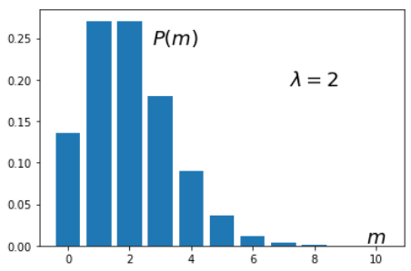 The distribution parameter $\lambda$ is usually determined from data analysis.
It represents the mean value $m_{avg}=\lambda$ and variance $D=\langle (m-m_{avg})^2 \rangle =\lambda$
(this follows as $n\to \infty$, $p\to 0$ from the statistics for the binomial distribution). The skewness is $\lambda^{-1/2}$
The larger $\lambda$, the more symmetrical the distribution will be around $m_{avg}$. For small $\lambda$
the distribution's peak approaches zero, and it has a long tail to the right (high asymmetry).
The distribution parameter $\lambda$ is usually determined from data analysis.
It represents the mean value $m_{avg}=\lambda$ and variance $D=\langle (m-m_{avg})^2 \rangle =\lambda$
(this follows as $n\to \infty$, $p\to 0$ from the statistics for the binomial distribution). The skewness is $\lambda^{-1/2}$
The larger $\lambda$, the more symmetrical the distribution will be around $m_{avg}$. For small $\lambda$
the distribution's peak approaches zero, and it has a long tail to the right (high asymmetry).
When using the Poisson distribution, events are usually observed over some time period $t$. Therefore, it is convenient to switch to the number of events per unit of time: $\lambda = np = \mu t$ (the longer $t$, the more observations $n$). The probability of observing $m$ events during time $t$ in this case is: $$ P(m) = \frac{(\mu t)^m}{m!}\,e^{-\mu t}. $$ No events will occur with a probability of $e^{-\mu t}$ during time $t$, and at least one event will occur with a probability of $1-e^{-\mu t}$.
Since $\langle m \rangle = \mu t$ during a small time interval $dt$, there will be $d\langle m \rangle = \mu \,dt$ events. Therefore, the distribution parameter $\mu = d\langle m \rangle \,/ \,dt$ is called the intensity of the Poisson process.
Normal distribution
✒ Let's now consider the limit of large $n$ and finite $p$ when $m\sim \,np=\langle m \rangle$ ($m$ is close to its mean value). First, let's find the expansion in $x$ of the factorial $(N+x)!$ when $N \gg x$. By definition: $$ \ln(N+x)! = \ln[N!(N+1)...(N+x)] = \ln N! + \sum^x_{k=1}\,\ln(N+k) = \ln N! + x\ln N + \sum^x_{k=1}\,\ln\Bigr(1+\frac{k}{N}\Bigr). $$ Taking into account the expansion $\ln(1+x)=x+...$ for small $x$ and the sum $1+2+...+x=x(x+1)/2$ (arithmetic progression), we finally get: $$ \ln(N+x)! = \ln N! + x\ln N + \frac{x(x+1)}{2N} + O\Bigr(\frac{1}{N^2}\Bigr). $$ It is worth noting that by setting $x=dN$, we can easily obtain the equation $d\ln(N!)/dN = \ln N + 1/2N$, from which the first three terms of Stirling's formula follow (up to a constant factor).
Now, let's introduce $x$, which is the deviation of $m$ from the mean value $np$. In this case, $m=pn + x$ и $n-m = qn - x$: $$ \ln P_n(m) = \ln n! - \ln(pn+x)! - \ln(qn-x)! + (pn+x)\,\ln p + (qn - x)\,\ln q. $$ Using the formula for $\ln(N+x)!$, we obtain: $$ \ln P_n(m) = \ln P_n(np) -\frac{x^2+(1-2p)\,x}{2D}, $$ where the first term corresponds to the constant terms of the expansion when $x=0$ and $D=n\,p\,q$ is the variance of the binomial distribution. The factor $1-2p$ in the linear term in $x$ varies in the range $(-1,...,1)$ and characterizes the asymmetry of the binomial distribution. This term makes a small contribution (and disappears when $p=1/2$). Indeed, since $x=1,2,3,...$ we have $x^2\gg (1-2p)\,x$ already for $x=2$ (for example, for $p=1/4$ we have $4 \gg 1$). The larger $x$, the smaller the contribution of this term.
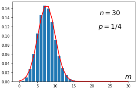 Thus, a good approximation to the binomial distribution for large $n$ and $p\sim 1/2$
is the normal distribution:
$$
P_n(m)\approx \frac{1}{\sqrt{2\pi D}}\,e^{-(m-np)^2/2D},
$$
where the normalization factor $1/\sqrt{2\pi D}$ is obtained by integrating over $x$ from $-\infty$ to $\infty$
(the exponential decays rapidly). This distribution is called "normal"
because it often arises in various practical problems. For example,
if the values of some quantity $X$ are measured, which is subject to a large number
of random and independent external influences, it becomes randomly distributed with a normal distribution.
Thus, a good approximation to the binomial distribution for large $n$ and $p\sim 1/2$
is the normal distribution:
$$
P_n(m)\approx \frac{1}{\sqrt{2\pi D}}\,e^{-(m-np)^2/2D},
$$
where the normalization factor $1/\sqrt{2\pi D}$ is obtained by integrating over $x$ from $-\infty$ to $\infty$
(the exponential decays rapidly). This distribution is called "normal"
because it often arises in various practical problems. For example,
if the values of some quantity $X$ are measured, which is subject to a large number
of random and independent external influences, it becomes randomly distributed with a normal distribution.
Useful integrals
When working with the normal distribution, we often encounter an integral of the following form:
$$
I = \int\limits^\infty_{-\infty} e^{-x^2} \,dx.
$$
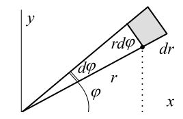 It is calculated in polar coordinates $(r,~\phi):~x=r\cos \phi,~~y=r\sin \phi$ as a double integral:
$$
I^2 = \int\limits^\infty_{-\infty} \int\limits^\infty_{-\infty} e^{-x^2-y^2} dx dy
= \int\limits_0^{2\pi} \int\limits^\infty_{0} e^{-r^2} r dr d\phi
= 2\pi \int\limits^\infty_{0} e^{-r^2} d\frac{r^2}{2} = \pi,
$$
where we took advantage of the fact that in coordinates $(r,~\phi)$ the area element equals the product of the arc $rd\phi$
and the change in radius $dr:~dxdy=rd\phi \, dr$.
Taking the square root and making the substitution $x \to x\sqrt{\alpha}$, we get:
$$
~I(\alpha) = \int\limits^\infty_{-\infty} e^{-\alpha x^2} dx = \sqrt{\frac{\pi}{\alpha}}.
$$
A useful technique is to differentiate both sides with respect to the parameter $\alpha$ to obtain integrals of even powers of $x^{2n}$.
The integral of odd powers of $x$ equals zero due to the antisymmetry of the integrand.
If we complete the square in the expression $-\alpha x^2+\beta x$, we get the following integral
(by using the substitution $x'=x-\beta/2\alpha$ it reduces to $I(\alpha)$ ):
$$
~\int\limits^\infty_{-\infty} e^{-\alpha x^2+\beta x} ~dx = \sqrt{\frac{\pi}{\alpha}}~ ~e^{\beta^2/4\alpha}.
$$
It is calculated in polar coordinates $(r,~\phi):~x=r\cos \phi,~~y=r\sin \phi$ as a double integral:
$$
I^2 = \int\limits^\infty_{-\infty} \int\limits^\infty_{-\infty} e^{-x^2-y^2} dx dy
= \int\limits_0^{2\pi} \int\limits^\infty_{0} e^{-r^2} r dr d\phi
= 2\pi \int\limits^\infty_{0} e^{-r^2} d\frac{r^2}{2} = \pi,
$$
where we took advantage of the fact that in coordinates $(r,~\phi)$ the area element equals the product of the arc $rd\phi$
and the change in radius $dr:~dxdy=rd\phi \, dr$.
Taking the square root and making the substitution $x \to x\sqrt{\alpha}$, we get:
$$
~I(\alpha) = \int\limits^\infty_{-\infty} e^{-\alpha x^2} dx = \sqrt{\frac{\pi}{\alpha}}.
$$
A useful technique is to differentiate both sides with respect to the parameter $\alpha$ to obtain integrals of even powers of $x^{2n}$.
The integral of odd powers of $x$ equals zero due to the antisymmetry of the integrand.
If we complete the square in the expression $-\alpha x^2+\beta x$, we get the following integral
(by using the substitution $x'=x-\beta/2\alpha$ it reduces to $I(\alpha)$ ):
$$
~\int\limits^\infty_{-\infty} e^{-\alpha x^2+\beta x} ~dx = \sqrt{\frac{\pi}{\alpha}}~ ~e^{\beta^2/4\alpha}.
$$
Let's calculate another integral by taking its derivative with respect to $\alpha$ $n$ times:
$$
I(\alpha) = \int\limits^\infty_{0} e^{-\alpha x} dx = -\frac{1}{\alpha}~e^{-\alpha x}\biggr|^{\infty}_0 = \frac{1}{\alpha}
~~~~~~~~~~~
\Rightarrow~~~~~~~~~~~~~\int\limits^\infty_{0} x^n e^{-\alpha x} dx = \frac{n!}{\alpha^{n+1}}.
$$
Integrals of this type are encountered frequently and a special notation has been introduced for them
in the form of a gamma function:
$$
~\Gamma(z) = \int\limits^\infty_{0} x^{z-1} e^{-x} dx.
$$
Integrating by parts, we see that $\Gamma(z+1)=z\,\Gamma(z)$.
In particular, for integer arguments: $\Gamma(n+1)=n!$.
For half-integer arguments, the gamma function reduces to the Gaussian integral. For instance, $\Gamma(1/2)=\sqrt{\pi}$.
Stirling formula follows from the integral definition of the gamma function. Let's represent $x^ne^{-x}$ as $e^{f(x)}$. The function $f(x)=-x+n \ln x$ has a maximum at $x_0=n$, since $f'(x_0)=-1+n/x_0=0$. Let's write its series in the vicinity of this point: $$ f(x)=f(n)+\frac{1}{2}\,f''(n)(x-n)^2+...~=~ -n + n\ln n - \frac{(x-n)^2}{2n}+... $$ Therefore, $$ n! \approx e^{-n + n \ln n} \int\limits^\infty_{0} e^{-\frac{(x-n)^2}{2n}} dx \approx e^{-n + n \ln n} \int\limits^\infty_{-\infty} e^{-\frac{(x-n)^2}{2n}} dx =e^{-n + n \ln n} \sqrt{2\pi n}. $$ In the second integral, the lower limit is replaced by $-\infty$, since for large $n$ the maximum of the exponential shifts far to the right and becomes increasingly narrow, so the integral from $-\infty$ to $0$ is practically zero. Hence the first three terms of the Stirling formula follow.
