ML: Probability Theory
Introduction
In machine learning and artificial intelligence tasks, probabilistic considerations play a significant role. For example, Bayesian methods are used in solving problems of classification and decision making. Markov models are widely used for natural language processing. Finally, concepts like cross-entropy form the basis of the most popular error functions when working with neural networks.
This paper is an informal introduction to probability theory and is the start of a series on the probabilistic approach to machine learning and artificial intelligence.
Joint and conditional probabilities
Let there be $N$ independent observations ( = trials) in which the event $A$ occurred $N(A)$ times and did not occur $N-N(A)$ times. The empirical probability $P(A)$ of the event $A$ is defined as the frequency of its occurrence: $$ P(A) = \frac{N(A)}{N}. $$ If two events $A$ and $B$ can occur in an observation, then the joint probability of both $A$ and $B$ occurring is defined as the ratio of the number of observations where both events occur $N(A,\,B)$ to the total number of observations $N$: $$ P(A\,\&\,B) \equiv P(A,\,B) = \frac{N(A,\,B)}{N}. $$
Let's consider the probability of the event $A$, occurring
if the event $B$ occurs in the same observation.
To do this, we need to count the number $N(A,\, B)$ of cases out of $N(B)$ observations where,
$B$ occurred.
Their ratio is called the conditional probability:
$$
P(B\to A) ~=~
\frac{N(A,\,B)}{N(B)} ~=~
\frac{P(A\,\&\,B)}{P(B)}.
$$
Usually, conditional probability is denoted as $P(A\mid B)$, but for our purposes, the notation
introduced above will be more convenient (especially in probabilistic logic
and Bayesian networks).
Conditional probability plays an important role in characterizing the degree of "correlation" between events $A$ and $B$. If whenever $B$ occurs, $A$ also occurs, then $P(B\to A)=1$. If, however, when $B$ occurs, the event $A$ never occurs, then $P(B\to A)=0$. The event $A$ is considered independent of $B$, when the conditional probability coincides with the regular one: $P(B\to A)=P(A)$. It is worth noting that if $P(A)\neq P(B)$, then $P(B\to A) \neq P(A\to B)$.
◊ A six-sided die is rolled onto the table (this is the observation) and one of the six numbers $\{1,2,3,4,5,6\}$ is obtained.
The event $A:$ "1 is rolled".
The event $B:$ "an odd number is rolled": $\{1,3,5\}$ (one of these numbers):
 $$
P(A) = \frac{1}{6},~~~~~~~~P(B) = \frac{1}{2},~~~~~~~~P(A\,\&\,B) = \frac{1}{6},
~~~~~~~P(B\to A) = \frac{1}{3},~~~~~~~P(A\to B) = 1.
$$
The probabilities are written under the assumption that the die is fair (symmetrical)
and all six numbers occur with equal frequency of $1/6$.
This means that with a large number of observations $N$, each number on the die will occur
approximately the same number of times, $N/6$.
The event $A\,\&\,B$ occurs only when $\{1\}$ is rolled,
and, for example, $P(B\to A)$ is defined as $P(A\,\&\,B)/P(B)=(N/6)/(N/2) = 1/3$.
$$
P(A) = \frac{1}{6},~~~~~~~~P(B) = \frac{1}{2},~~~~~~~~P(A\,\&\,B) = \frac{1}{6},
~~~~~~~P(B\to A) = \frac{1}{3},~~~~~~~P(A\to B) = 1.
$$
The probabilities are written under the assumption that the die is fair (symmetrical)
and all six numbers occur with equal frequency of $1/6$.
This means that with a large number of observations $N$, each number on the die will occur
approximately the same number of times, $N/6$.
The event $A\,\&\,B$ occurs only when $\{1\}$ is rolled,
and, for example, $P(B\to A)$ is defined as $P(A\,\&\,B)/P(B)=(N/6)/(N/2) = 1/3$.
☝ The requirement of independent trials means that the outcomes of a given trial
are not dependent on the outcomes of previous ones. It is said that the trials should be conducted under the same (but not identical!) conditions.
For example, to obtain $P(A)=1/6$, where $A:$ "a one is rolled on the die",
the "fair die" must also be rolled "fairly", i.e. to conduct a random experiment.
This creates a vicious circle in defining the random nature of each trial,
and a random experiment is only a mathematical model of physical reality.
☝ A trial does not necessarily consist of a single action. For example, let's say a coin with $0$ written on one side and $1$ on the other is flipped five times. One trial would be a sequence like $01001$. There are a total of $2^5 = 32$ possible outcomes of the trials. If the coin is "fair" (symmetrical) and the method of flipping it is "fair", then all sequences are equally probable. In particular, $00000$ will occur with the same frequency ($P=1/32$) as, for example, $10101$. Although the event $A$: "the number of zeros in the sequence is equal to $3$ or $2$" will occur $20$ times more often than the event $B$: "falls out $00000$". At the same time, $A$ and $B$ are mutually exclusive events, meaning they never occur simultaneously: $P(A\,\&\,B) = 0$. It is worth listing all $32$ combinations and counting the number of those favorable to the event $A$.
Another example is flipping a coin until the number of zeros equals the number of ones. In this case, the outcomes of the trials will be variable-length sequences like $01$ or $001011$, but not $0101$.
☝ It is important to remember that the conjunction of events $A\,\&\,B$ does not imply their simultaneity. For example, let's say two dice of different colors are rolled on the table $N$ times, where the event $A$ denotes a six on the green die and the event $B$: one on the blue die. The probability $P(A\,\&\,B)=1/36$ does not depend on whether the dice are rolled simultaneously or sequentially (considering both dice being on the table after the roll/rolls as one observation).
Similarly, the conditional probability $P(B\to A)$ does not imply that the event $B$ occurs before the event $A$. For instance, the event $B$ could be getting a 1 on the second die rolled, and the event $A$ could be getting a 6 on the first die.
☝ The term "empirical probability" implies that the ratio $N(A)/N$ merely serves as an estimate of the "true" probability. This estimation becomes more accurate as $N$ increases. Let the "true" probability (based on an "infinite" number of observations) be equal to $p_A$. Then, the variance of the empirical probability based on $N$ observations equals $p_A\,(1-p_A)/N$, and the measurement error in probability decreases relatively slowly as $N$ grows: $$ P(A) ~=~ \frac{N(A)}{N} ~\pm~ \sqrt{\frac{p_A\,(1-p_A)}{N}}. $$
The "true" (mathematical) probability $p_A$ is an abstraction, assuming that each event possesses such a numerical characteristic. However, in the macro world, it's a bit of a "spherical cow". They exist with a stretch for symmetric processes (coin flips, roulette). Although in practice, the stationarity (time invariance) of empirical probabilities is rarely achieved. It's worth recalling, for example, the successes of Smoke Bellew while playing roulette.
"Strict mathematics" prefers axiomatic definition to the frequency definition of probability, where probabilities of elementary events are specified, and then probabilities of composite events are calculated with all rigor. However, in the real world, a balance between rigor and practicality is necessary.
Probabilities, logic, and set theory
Many relationships in probability theory can be easily derived using geometric considerations. Let's represent all conducted experiments as identical squares inside a square of unit area, which we'll call the sample space. We'll mark experiments in which event $A$ occurs as the shaded area $A$ (see the first figure below). Experiments not falling into this area correspond to the event where "$A$ did not occur" or "not $A$". We'll denote them in logical notation as $\neg A$ or with a bar over: $\bar{A}$. It's clear that the probability (area) of "not $A$" is equal to $P(\bar{A}) = 1 - P(A)$. Notice that the converse is not true: from $P(B)=1-P(A)$, it does not follow that $B=\bar{A}$ (construct a disproving picture).
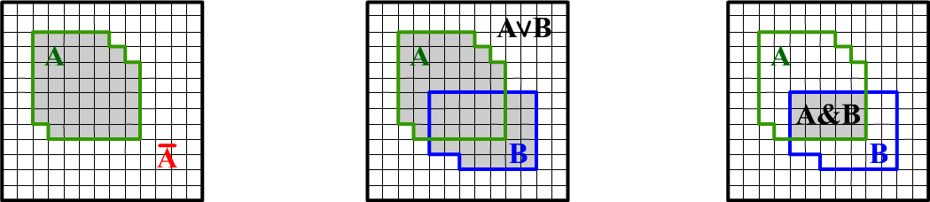
If an experiment yields either $A$, or $B$, or both events, then the probability $P(A\vee B)$ or $P(A\cup B)$ equals the shaded area encompassing both events (second figure). The logical notation $A\vee B$ and set-theoretic $A \cup B$ are equivalent. In the former case, we emphasize that the assertion about the occurrence of events is formed using the logical OR operator. In the latter, it signifies that the sets of experiments in which these events occur are combined. We'll more often use logical notations.
The occurrence of two events $A$ and $B$ in one experiment corresponds to the shaded area in the third figure. This intersection of events is $A \cap B$. The area of this region equals the joint probability $P(A\,\&\,B)$, or simply $P(A,\,B)$. The third figure also illustrates the definition of conditional probability $P(B\to A)=P(A\,\&\,B)/P(B)$. If it's known that event $B$ occurred, then the entire sample space "contracts" to the area $B$, and for event $A$, only the experiments within $B$ need to be considered.
Relations between probabilities
✒ Let's find the probability of the union of two events (logical OR). The area $P(A\vee B)$ equals the sum of the area $P(A)$, $P(B)$, minus the area of their intersection $P(A\,\&\,B)$, which is counted twice when adding up the areas: $$ P(A\vee B) = P(A) + P(B) - P(A\,\&\,B). $$
Substituting the negation $\bar{A}$ for $B$, we obtain $P(\bar{A}) = 1 - P(A)$. Here, $A\vee\bar{A}=\mathbb{T}$ - this is the entire sample space (a square of unit area), and $A\,\&\,\bar{A}=\mathbb{F}$ - the impossible event, which has zero probability.
✒
 In logic, the disjunction (OR) and conjunction (AND) are related by De Morgan's law:
$$
~~~~~~~~~~~~~~~~~~~~~~~\neg(A\vee B)=\neg A\,\&\,\neg B
~~~~~~~~\text{ or }~~~~~~~~~~~~
A\vee B=\neg( \bar{A}\,\&\,\bar{B}).
$$
From it follows another important relation for the probability of union of events:
$$
~~~~~~~~~~~~~~~~~~~~~~~~~P(A\vee B) = 1 - P\bigr(\bar{A}\,\&\,\bar{B}\bigr).
$$
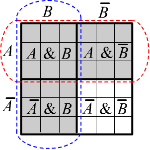
Its illustration is provided in the figure on the right.
The horizontally striped area outlined in red represents event $A$.
The vertically striped area outlined in blue represents event $B$.
Their union $A\vee B$ is shaded in gray. The remaining unshaded part represents the negation of
$A\vee B$ which is also equal to $\bar{A}\,\&\,\bar{B}$.
This formula is convenient for computing the union of a large number of events:
$$
P(A_1\vee ...\vee A_n) ~=~ 1 - P(\bar{A}_1\,\&\, ...\,\&\, \bar{A}_n).
$$
In logic, the disjunction (OR) and conjunction (AND) are related by De Morgan's law:
$$
~~~~~~~~~~~~~~~~~~~~~~~\neg(A\vee B)=\neg A\,\&\,\neg B
~~~~~~~~\text{ or }~~~~~~~~~~~~
A\vee B=\neg( \bar{A}\,\&\,\bar{B}).
$$
From it follows another important relation for the probability of union of events:
$$
~~~~~~~~~~~~~~~~~~~~~~~~~P(A\vee B) = 1 - P\bigr(\bar{A}\,\&\,\bar{B}\bigr).
$$
Its illustration is provided in the figure on the right.
The horizontally striped area outlined in red represents event $A$.
The vertically striped area outlined in blue represents event $B$.
Their union $A\vee B$ is shaded in gray. The remaining unshaded part represents the negation of
$A\vee B$ which is also equal to $\bar{A}\,\&\,\bar{B}$.
This formula is convenient for computing the union of a large number of events:
$$
P(A_1\vee ...\vee A_n) ~=~ 1 - P(\bar{A}_1\,\&\, ...\,\&\, \bar{A}_n).
$$
✒ Using the figure above, it is easy to verify that $P(A\vee B)=P(A)+P(\bar{A}\,\&\,B)$.
The generalization of this relation is called the orthogonal decomposition of disjunction:
$$
P(A_1\vee ...\vee A_n) ~=~ P(A_1) + P(\bar{A}_1,A_2)+...+P(\bar{A}_1,...,\bar{A}_{n-1},A_n).
$$
It is proved by induction using the previous relation ($n=2$).
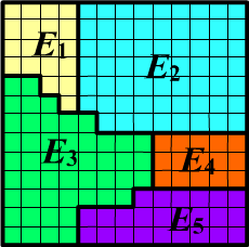
 ✒ Consider a set $\{H_1,...,H_n\}$ of non-intersecting events: $H_i\,\&\,H_j=\mathbb{F}\equiv\varnothing$,
which are called mutually exclusive. For such events, the following relation
holds:
$$
P(H_1\vee H_2\vee...\vee H_n) = P(H_1)+P(H_2)+...+P(H_n).
$$
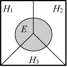
Let the mutually exclusive events cover the entire sample space by partitioning it (see the example for $n=3$ on the right).
In this case, the normalization condition is satisfied:
$$
\sum_iP(H_i) = 1.
$$
Additionally, for any event $E$
the law of total probability holds:
$$
P(E) = \sum_i P(H_i \,\&\, E) = \sum_i P(H_i)\,P(H_i\to E),
~~~~~~~~~~~~~~~~~~
$$
where the definition of conditional probability is taken into account. In a special case, for any two events:
$$
P(A) ~=~ P(A,\,B)+P(A,\,\bar{B}) ~=~ P(B)\,P(B\to A)\,+\,P(\bar{B})\,P(\bar{B}\to A),
$$
where $B$ and $\bar{B}$ partition the entire sample space into two non-intersecting areas.
✒ Consider a set $\{H_1,...,H_n\}$ of non-intersecting events: $H_i\,\&\,H_j=\mathbb{F}\equiv\varnothing$,
which are called mutually exclusive. For such events, the following relation
holds:
$$
P(H_1\vee H_2\vee...\vee H_n) = P(H_1)+P(H_2)+...+P(H_n).
$$
Let the mutually exclusive events cover the entire sample space by partitioning it (see the example for $n=3$ on the right).
In this case, the normalization condition is satisfied:
$$
\sum_iP(H_i) = 1.
$$
Additionally, for any event $E$
the law of total probability holds:
$$
P(E) = \sum_i P(H_i \,\&\, E) = \sum_i P(H_i)\,P(H_i\to E),
~~~~~~~~~~~~~~~~~~
$$
where the definition of conditional probability is taken into account. In a special case, for any two events:
$$
P(A) ~=~ P(A,\,B)+P(A,\,\bar{B}) ~=~ P(B)\,P(B\to A)\,+\,P(\bar{B})\,P(\bar{B}\to A),
$$
where $B$ and $\bar{B}$ partition the entire sample space into two non-intersecting areas.
✒ The next important relation is called the chain rule:
$$
P(A_1,A_2,...,A_n) = P(A_1)\cdot P(A_1\to A_2)\cdot P(A_1,A_2\to A_3)\cdot...\cdot P(A_1,...,A_{n-1}\to A_n).
$$
It is easy to prove by substituting the definitions $P(A_1,A_2\to A_3)=P(A_1,A_2, A_3)/P(A_1,A_2)$, etc.
The chain rule can be interpreted as follows:
for events $A_1,...,A_n$ to occur simultaneously in an experiment, it is necessary for $A_1$ to happen first;
if this occurs, then $A_2$ must happen, i.e. $A_1\to A_2$, and so on.
It is clear that the order in which events are chosen for the chain rule can be arbitrary.
✒ (*) In conclusion, we present the formula for the disjunction of $n$ events: $$ P(A_1\vee A_2\vee...\vee A_n) = \sum^n_{i=1} P(A_i) - \sum_{1 \le i\lt j\le n} P(A_i,A_j) + \sum_{1 \le i\lt j \lt k\le n} P(A_i,A_j,A_k) - ... +(-1)^{n+1} P(A_1,A_2,...,A_n). $$ It is proven by induction, using the relation $P(A\vee B)=P(A)+P(B)-P(A,B)$ (case $n=2$), where $A=A_1\vee...\vee A_n$ и $B=A_{n+1}$ are set. Then, it is necessary to consider the distributivity of disjunction and conjunction $(A_1\vee...\vee A_n)\,\&\,A_{n+1}=(A_1\,\&\,A_{n+1})\,\vee...\vee\, (A_n\,\&\,A_{n+1})$ and the absorption law $A_{n+1}\,\&\,A_{n+1}=A_{n+1}$.
A few inequalities *
✒ Using the formula for the total probability $P(A) = P(A\,\&\,B) + P(A\,\&\,\bar{B})$ and the positivity of probabilities, we conclude that $P(A) ~\ge~ P(A\,\&\,B)$ and a similar inequality for $B$. Additionally, from $A\,\&\,B=\neg\neg(A\,\&\,B)$ or $$P(A\,\&\,B)=1-P(\neg(A\,\&\,B))=1-P(\bar{A}\vee \bar{B})= 1-P(\bar{A})-P(\bar{B})+P(\bar{A}\,\&\,\bar{B})= P(A)+P(B)-1+P(\bar{A}\,\&\,\bar{B}), $$ it follows that $P(A\,\&\,B)$ is greater than $P(A)+P(B)-1$. As a result, we obtain the following constraint on the probability of the joint occurrence of two events (see also the illustration on the right):
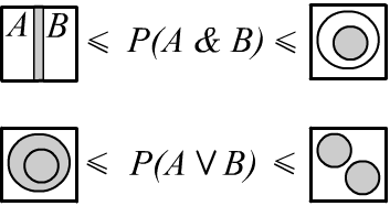 $$
\max[0,~P(A)+P(B)-1]~~~\le~~~ P(A\,\&\,B) ~~~\le~~~ \min[P(A),\,P(B)].~~~~~~~~~~~
$$
$$
\max[0,~P(A)+P(B)-1]~~~\le~~~ P(A\,\&\,B) ~~~\le~~~ \min[P(A),\,P(B)].~~~~~~~~~~~
$$
Similarly, for the range of the probability of the union of two events: $$ \max[P(A),\,P(B)]~~~~~~~~\le~~~~~~ P(A\vee B) ~~~\le~~~\min[1,~P(A)+P(B)]. $$
The sample space is quite "tight", so if $P(A)$ or $P(B)$ significantly differ from $1/2$ (preferably both in the same direction), then these inequalities provide narrow intervals for the conjunction ($\&$) and disjunction ($\vee$). In various versions of fuzzy logic, upper or lower bounds of these intervals are used to estimate the conjunction and disjunction of two fuzzy propositions. Naturally, the inequalities do not account for possible dependencies between events. For example, if $B=\bar{A}$, then $P(A\,\&\,B)=0$ is at the lower bound of the interval, and $P(A\vee B)=1$ is at the upper bound.
| $P(A)$ | $P(B)$ | $P(A\,\&\,B)$ | $P(A\vee B)$ |
| $0.5$ | $0.9$ | $[0.4,\,0.5]$ | $[0.9,\,1.0]$ |
| $0.5$ | $0.1$ | $[0.0,\,0.1]$ | $[0.5,\,0.6]$ |
| $0.3$ | $0.7$ | $[0.0,\,0.3]$ | $[0.7,\,1.0]$ |
| $0.5$ | $0.5$ | $[0.0,\,0.5]$ | $[0.5,\,1.0]$ |
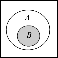 ✒ Let's consider the relation $P(A\,\&\,B)\,=\,P(B)$.
Then the event area of $B$
is a subset ($B\subset A$) of the event area of $A$. In this case:
$$
P(B) \le P(A) \le 1.
$$
From the definition $P(B\to A)=P(A\,\&\,B)/P(B)$, it follows that $P(B\to A)=1$.
This means that whenever event $B$ occurs, event $A$ will definitely occur as well
($B$ entails $A$).
✒ Let's consider the relation $P(A\,\&\,B)\,=\,P(B)$.
Then the event area of $B$
is a subset ($B\subset A$) of the event area of $A$. In this case:
$$
P(B) \le P(A) \le 1.
$$
From the definition $P(B\to A)=P(A\,\&\,B)/P(B)$, it follows that $P(B\to A)=1$.
This means that whenever event $B$ occurs, event $A$ will definitely occur as well
($B$ entails $A$).
✒ Let's prove another inequality that finds application in probabilistic logic: $$ P(A\to B)~~\le~~P(\bar{A}\vee B). $$ Using the formula for disjunction and the total probability $P(B)=P(A,B)+P(\bar{A},B)$ we have: $$ P(\bar{A}\vee B)=P(\bar{A})+P(B)-P(\bar{A},B)=1-P(A)+P(A,B)+P(\bar{A},B)-P(\bar{A},B) = 1-P(A)\,\bigr(1-P(A\to B)\bigr). $$ This implies $1-P(\bar{A}\vee B) = P(A)\,\bigr(1-P(A\to B)\bigr)$, and since, $P(A)\le 1$, we obtain the required inequality.
Set of elementary events
 An event is called elementary
if it cannot be represented as the union of other events.
An event is called elementary
if it cannot be represented as the union of other events.
In this experiment, one and only one elementary event
always occurs (they are all pairwise disjoint, and one of them will definitely occur).
The set of elementary events $\{E_1,...,E_n\}$
is denoted by the letter $\Omega$. In this case, $P(\Omega)=1$ и $P(E_i\, \&\, E_j)=0,~i\neq j$.
Any event $A$ is a subset of the set of elementary events: $A\subset \Omega$.
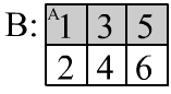
◊ Arbitrary events can intersect. For example, for $\Omega=\{E_1,E_2,E_3,E_4,E_5\}$ and compound events $A=\{E_1,E_3,E_5\}$, $B=\{E_1,E_2,E_3\}$ we have $A\,\&\,B=\{E_1,E_3\}$. The curly brackets for $A\,\&\,B$ in this case denote the exclusive logical OR (either $E_1$ occurred, or $E_3$).
In probability theory a problem is fully defined if the set of elementary events is known and their probabilities are specified. It is assumed that the procedure for specifying these probabilities lies outside the theory.
◊ Let's assume that in the above example, the probabilities of elementary events are specified as $\{P_1,\,P_2,\,P_3,\,P_4,\,P_5\}$, whose sum equals one. Then $P(A)=P_1+P_3+P_5$, а $P(A\,\&\,B)=P_1+P_3$.
☝ Let's emphasize the difference between elementary events and an arbitrary partition of the sample space. Elementary events divide the space in such a way that any event can be expressed as a union of them. The set $\Omega$ with $|\Omega| = n$ elements has $2^{n}$ subsets (including the empty set $\varnothing$ and $\Omega$ itself). This set of subsets is denoted as: $2^{\Omega}$. To number subsets you can use binary numbers like $10101$, which, for the example above, represent $A=\{E_1,E_3,E_5\}$.
A set of arbitrary events, in turn, generates a set of elementary events. For example, if only events $A$ and $B$ can occur in the experiments, then the set of elementary events will consist of four elements $\{ A\,\&\,B,~A\,\&\,\bar{B},~\bar{A}\,\&\,B,~\bar{A}\,\&\,\bar{B}\}$, where the absence of events $\bar{A}\,\&\,\bar{B}$ in the experiment is also considered an event. If some of these combinations are impossible, then the set of elementary events decreases. In general, $n$ events can generate no more than $2^n$ pairwise disjoint elementary events.
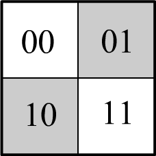 ◊ Two coins of different sizes are tossed onto a table (simultaneously or sequentially).
Then the set of elementary events is $\Omega = \{00,\, 01,\, 10,\, 11\}$, where
$0$ stands for "heads" and $1$ - for "tails," with the first digit representing the outcome of the smaller coin, for instance.
Due to symmetry considerations, for fair coins and tossing methods,
the probabilities of all four elementary events are equal to $1/4$.
◊ Two coins of different sizes are tossed onto a table (simultaneously or sequentially).
Then the set of elementary events is $\Omega = \{00,\, 01,\, 10,\, 11\}$, where
$0$ stands for "heads" and $1$ - for "tails," with the first digit representing the outcome of the smaller coin, for instance.
Due to symmetry considerations, for fair coins and tossing methods,
the probabilities of all four elementary events are equal to $1/4$.
If the coins are identical and indistinguishable, the set of elementary events consists of three elements: $\Omega = \{00,\, 01,\, 11\}$ (two heads, one head and one tail, two tails). In this case, $P(00)=P(11)=1/4$ and $P(01)=1/2$, where the latter probability represents the probability of the union of the elementary events the probability of the union of the elementary events $01,\, 10$ for distinguishable coins into a single elementary event for indistinguishable coins.
Note that this "obvious" reasoning was not apparent in the early days of probability theory. It was then believed that for identical coins, the elementary events $\{00,\, 01,\, 11\}$ should be equiprobable ($1/3$). In reality, the fact that indistinguishable coins "can be distinguished in principle" and the probability $P(01 \vee 10)=1/2$, rather than $1/3$, is a physical (experimental) fact. While valid in the macro world, this does not hold true in the micro world, which is reflected in the difference between Bose and Maxwell statistical distributions.
 ◊ In a closed urn, there are four white ($w$) and one black ($b$) ball.
First, one ball is randomly selected, and then another (balls are not returned to the urn).
One trial is a sequence
and there are four possible elementary events:
$\Omega = \{ w_1w_2,\,w_1b_2,\,b_1w_2,\,b_1b_2 \}$ (first white, then white again, and so forth).
Their probabilities are:
$$
P(w_1w_2) = \frac{4}{5}\,\frac{3}{4}=\frac{3}{5},~~~~
P(w_1b_2) = \frac{4}{5}\,\frac{1}{4}=\frac{1}{5},~~~~
P(b_1w_2) = \frac{1}{5}\,1=\frac{1}{5},~~~~
P(b_1b_2) = \frac{1}{5}\,0=0.
$$
Indeed, the probability of drawing a white ball first is $P(w_1)=4/5$.
Then, there are 3 white balls and 1 black left in the urn. The probability of drawing another white ball is $P(w_1\to w_2)=3/4$.
By the definition of conditional probability, $P(w_1,w_2)=P(w_1)\,P(w_1\to w_2)$, which gives $(4/5)\cdot(3/4)$. Similarly for the other scenarios.
◊ In a closed urn, there are four white ($w$) and one black ($b$) ball.
First, one ball is randomly selected, and then another (balls are not returned to the urn).
One trial is a sequence
and there are four possible elementary events:
$\Omega = \{ w_1w_2,\,w_1b_2,\,b_1w_2,\,b_1b_2 \}$ (first white, then white again, and so forth).
Their probabilities are:
$$
P(w_1w_2) = \frac{4}{5}\,\frac{3}{4}=\frac{3}{5},~~~~
P(w_1b_2) = \frac{4}{5}\,\frac{1}{4}=\frac{1}{5},~~~~
P(b_1w_2) = \frac{1}{5}\,1=\frac{1}{5},~~~~
P(b_1b_2) = \frac{1}{5}\,0=0.
$$
Indeed, the probability of drawing a white ball first is $P(w_1)=4/5$.
Then, there are 3 white balls and 1 black left in the urn. The probability of drawing another white ball is $P(w_1\to w_2)=3/4$.
By the definition of conditional probability, $P(w_1,w_2)=P(w_1)\,P(w_1\to w_2)$, which gives $(4/5)\cdot(3/4)$. Similarly for the other scenarios.
Placing $M$ white balls and $N-M$ black balls in the urn, it's worth noting that $P(w_1,b_2)=P(b_1,w_2)$. This should be the case because the color of the drawn balls can be observed at the end (by shuffling them).
If we are only interested in the second ball, we can sum the probabilities of elementary events based on the first ball: $P(w_2)=P(w_1,\,w_2)+P(b_1,\,w_2)=4/5$ = the probability of drawing a second white ball. The conditional probability of drawing a black ball first, given that the second ball was white, is $P(w_2\to b_1) = P(b_1,\,w_2)/P(w_2)=1/4$.
◊ There are two urns. In the first urn, there are $5$ balls, of which $4$ are white and $1$ is black. In the second urn, there are $2$ white and $2$ black balls. Two balls are randomly chosen from the first urn and transferred to the second urn. What is the probability of then drawing a white ball from the second urn?
Let $w_1b_2w$ denote that a white ball ($w_1$) was first drawn from the first urn, then a black one ($b_2$). They were transferred to the second urn, from which a white ball ($w$) was then drawn. The set of elementary events consists of eight elements: $\Omega=\{w_1w_2w,\,w_1b_2w,\,b_1w_2 w,\,b_1b_2 w,\,w_1w_2b,\,w_1b_2b,\,b_1w_2 b,\,b_1b_2 b\}$. The probabilities of these events are calculated using the chain rule: $P(x_1x_2x)=P(x_1)P(x_1\to x_2)P(x_1,x_2\to x)$. As a result, $P=\{4,\,1,\,1,\,0,\,2,\,1,\,1,\,0\}/10$. The sum (union) of the first four events favors the drawing of a white ball at the end, with a probability of $6/10=3/5$.
◊ It is known that someone won one of three possible prizes in a lottery: $W_1,W_2,W_3$.
The probabilities of such winnings are $P(W_i)$, and $P_0$ is the probability of losing.
What is the probability that the third prize was won?
The set of elementary events consists of $\{W_0,W_1,W_2,W_3\}$. We need to calculate
the conditional probability:
$$
P(W_1\vee W_2\vee W_3 \to W_3)= \frac{P\bigr((W_1\vee W_2\vee W_3) \,\&\, W_3\bigr)}{P(W_1\vee W_2\vee W_3)}=\frac{P(W_3)}{P(W_1)+P(W_2)+P(W_3)}.
$$
Since the elementary events are mutually exclusive, it is taken into account that $W_1\,\&\,W_3=W_2\,\&\,W_3=\varnothing$ and $W_3\,\&\,W_3=W_3$.
Probability tables
Let's denote the event by a capital letter $A$, and by lowercase letters $a,\bar{a}$ - its two possible "values": $A=a$ - the event occurred, and $A=\bar{a}$ - it did not occur. Then the probabilities $P(a)$ and $P(\bar{a})=1-P(a)$ will be numbers, and $P(A)$ - a vector with components $\{P(a),P(\bar{a})\}$ or a function into which $a$ or $\bar{a}$ must be substituted.
Let's consider that, in the general case, we are interested in $n$ events $\{X_1,...,X_n\}$. Then $2^n$ probabilities $P(X_1,...,X_n)$, where $X_i = x_i$ (event occurs) or $X_i = \bar{x}_i$ (event does not occur) completely determine the problem. Each such probability characterizes an elementary event. Knowing these numbers, one can answer any question. For example, the probability $P(X_1,X_2)$ is equal to the sum of $P(X_1,...,X_n)$ over possible "values" of events $X_3,...,X_n$ and so on.
| $s$ | $\bar{s}$ | Tot | |
|---|---|---|---|
| $b$ | 8 | 2 | 10 |
| $\bar{b}$ | 32 | 58 | 90 |
| Tot | 40 | 60 | 100 |
In the notations introduced above, $P(b\to S)$ is a function of $S$ with 2 values for $S=s$ and $S=\bar{s}$: $$ P(b\to S) ~=~ \bigr\{ p(b \to s),~~~p(b\to \bar{s})\bigr\} ~=~ \bigr\{ 8,~~~2\bigr\}/10. $$ At the same time, $P(B\to S)$ is already a $2\times 2$ matrix with components $P(b\to s)$, $P(b\to \bar{s})$, $P(\bar{b}\to s)$, $P(\bar{b}\to \bar{s})$.
Let's find the probability that the encountered person is neither blonde nor smart. From a logical point of view, $\bar{B} \vee S = \neg\neg(\bar{B}\vee S) = \neg(B\,\&\,\bar{S})$. Therefore: $$ P(\bar{b} \vee s ) = 1- P(b,\,\bar{s}) = 1-\frac{2}{100} = 0.98. $$ This result can also be obtained using the identity: $$ P(\bar{b} \vee s) = P(\bar{b}) + P(s) - P(\bar{b},\, s) = \frac{90}{100} + \frac{40}{100} - \frac{32}{100} = \frac{98}{100} $$ or simply by summing the corresponding numbers of events: $(32+58+8)/100$ from the second row and the first column (without repetitions).
Random variables
Let the variable $X$ take one of the values belonging to a certain set in each trial. If the set is countable, for example, $\{x_1,...,x_n\}$, then $X$ is called a discrete random variable. If the values of $X$ are real numbers, then it is a continuous random variable.
◊ Rolling a die can be considered as a discrete random variable with six possible values $X=x \in\{1,2,3,4,5,6\}$. The point on the table where the die lands is a continuous vector random variable with two components $\mathbf{X}=\mathbf{x}=\{x_1,x_2\}$ (the coordinates of the die).
Random variables are typically denoted by uppercase letters such as $X$, and their values are denoted in lowercase $x$. The probabilities with which values appear in a trial are called probability distributions (discrete or continuous): $P(X=x)$. This is briefly expressed as a function $p(x)$.
An event is a special case of a discrete random variable with two values ($1$ - the event occurred or $0$ - the event did not occur). Instead of writing $P(A=1)$ above, we wrote $P(a)$, and for $P(A=0)$ - $P(\bar{a})$. The set of elementary events $E=e \in \Omega=\{E_1,...,E_n\}$ is a random variable (in this trial, exactly one event occurs, i.e., $E$ has a specific value from the set $\Omega$). On the other hand, a discrete random variable can be considered as an event with two mutually exclusive outcomes: $P(X=x)$ или $P(X\neq x)$.
Since a random variable takes a specific value in each trial, the sum of the probability distribution must equal one. This normalization condition is expressed differently for discrete and continuous variables: $$ \sum_i p(x_i)=1,~~~~~~~~~~~~~~~~~~~~~~\int\limits_X p(x)\,dx = 1. $$ In the second case, the function $p(x)$ is called the probability density, and $p(x)\,dx$ represents the probability that the random variable falls within the range $[x,\,x+dx]$. Integration is performed over the entire range of possible values for $X$. For brevity, we will refer to discrete variables. In the case of continuous random variables, all formulas need to replace $p(x_i)$ with $p(x)\,dx$, and the sum with an integral.
✒ The mean $X_\text{mean}$ of a random variable is the weighted sum of its possible values by their probabilities. The averaging of squares of deviations from the mean is called the variance $D$: $$ X_\text{mean}\equiv \langle X \rangle = \sum_i x_i\, p(x_i),~~~~~~~~~~~~D = \langle (X-X_\text{mean} )^2 \rangle = \sum_i (x_i-X_\text{mean})^2\, p(x_i). $$ The more likely a value of the random variable, the greater its contribution to the mean. If the probability distribution $p(x)$ has a single symmetric peak, then the mean characterizes its location, and the square root of the variance $\sigma=\sqrt{D}$ (standard deviation) represents the width of the peak.
Directly from the definition, it follows that the variance can also be computed using this formula: $$ D = \langle (X-X_\text{mean} )^2 \rangle = \langle X^2-2X\,X_\text{mean}+X^2_\text{mean} \rangle =\langle X^2\rangle-2\langle X\rangle\,X_\text{mean}+X^2_\text{mean} = \langle X^2\rangle - X^2_\text{mean}, $$ where it is considered that the mean of a sum is equal to the sum of means, and the constant factor (constant) $X_\еуче{mean}$ can be moved outside the mean sign (outside the sum). Note that if $D \neq 0$, then the mean square of a random variable is not equal to the square of its mean: $$ \langle X+Y\rangle = \langle X\rangle + \langle Y\rangle,~~~~~~~~~ \langle \alpha\,X\rangle = \alpha\,\langle X\rangle,~~~~~~~~~ \langle X^2\rangle \neq \langle X\rangle^2. $$
◊ A die is rolled until a $6$ appears. Calculate the average number of rolls in such an experiment.
The random variable $N$ represents the number of rolls.
The probability of getting $n-1$ non-sixes followed by a six is $(5/6)^{n-1}(1/6)$.
Therefore, the average length is
(using the summation of the infinite series $x^n$, which equals $1/(1-x)$, and its derivative $n\, x^{n-1}$,
the sum of which is $1/(1-x)^2$):
$$
N_{mean} = \sum^\infty_{n=1} n\, \left(\frac{5}{6}\right)^{n-1}\,\frac{1}{6} = 6.
$$
There's an elegant argument
that doesn't require summation.
The results of $K$ experiments are "spliced" into one sequence like
$4125\mathbf{6}115323\mathbf{6}...$
Sixes in it will occur with a probability of $1/6$, so the length $L$ of the sequence
is $6\cdot K$, and the average length of one experiment is: $L/K=6$.
Independence of events
Events $A,B$ are called independent, if the conditional probability of $A$ does not depend on whether event $B$ occurs, and the probability of $B$ does not depend on the occurrence of $A$: $$ P(B \to A)=P(A),~~~~~~~~~~~~~P(A \to B)=P(B). $$ If in $N$ trials we are not interested in $B$, then $P(A)=N(A)/N$. If, however, we only select those trials in which $B$ occurs, then $P(B\to A)=N(A,\,B)/N(B)$. When these two quantities coincide, it means that the probability of $A$ does not depend on whether we are interested in $B$ or not (= $A$ is independent of $B$).
From the definition of conditional probability, it follows that the joint probability
of independent events is:
$$
P(A,\,B)=P(A)\cdot P(B).
$$
Independence of events is denoted as follows: $A\Prep B$
(the joint probability "splits").
If $P(A,\,B,\,C)=P(A)\cdot P(B)\cdot P(C)$, then this is $A\Prep B \Prep C$ (three independent events).
It is obvious that mutually exclusive events $P(A,B)=0$ are always independent, provided that $P(A),P(B) \gt 0$.
☝ Sometimes independence is intuitively obvious when there is no connection between events (for example, when flipping two coins). However, it can also be a "random" effect of statistics. For example, suppose there are 100 women in the universe. Among them, 10 are blond $(B)$ and 20 have green eyes ($G$). If there are 2 green-eyed blondes, then the events $B$ and $G$ will be independent. With a different number of $B\,\&\,G$, this is no longer the case.
In general, "dependence" (failure to satisfy the condition of independence) $P(A,\,B)\neq P(A)\cdot P(B)$ should not be understood in the ordinary sense. In particular, the fact of "dependence" does not mean that $A$ is the cause of $B$ or vice versa. It is better to think of independence in terms of conditional probability $P(A\to B)=P(B)$: "Does knowledge of the value of $A$ add anything to predicting the value of $B$?".
◊ Consider three events that occur when rolling a die, where "the number that comes up is ...":
$$
\text{"even": } A=\{2,4,6\};~~~~~~~ \text{"divisible by three":} B=\{3,6\};~~~~~~~\text{"less than five": }C=\{1,2,3,4\}.
$$
Since $A\,\&\,B = \{6\}$, $A\,\&\,C = \{2,4\}$, $B\,\&\,C = \{3\}$, it is easy to verify that $A\Prep B$, $A\Prep C$,
but $B$ and $C$ are not independent.
 ✒ Let two events be independent $A\Prep B$.
Will their negations $\bar{A}\Prep \bar{B}\,$ also be independent?
✒ Let two events be independent $A\Prep B$.
Will their negations $\bar{A}\Prep \bar{B}\,$ also be independent?
Yes, they will be. Let's use geometric reasoning. The set of elementary events
in the sample space is shown on the right.
The event $A\,\&\,B$ (upper left corner) has a probability ("area") of
$P(A)\,P(B)$. The entire top row with an area of $P(A)$ corresponds to the event $A$.
Therefore, the event $A\,\&\,\bar{B}$ has an area of $P(A)-P(A)\,P(B)$. Similarly, for the remaining two
elementary events $\bar{A}\,\&\,B$ и $\bar{A}\,\&\,\bar{B}.$
✒ Joint probabilities of independent events factorize as $P(A,\,B)=P(A)\,P(B)$. However, pairwise fulfillment of this relationship among a set of events does not always imply their independence.
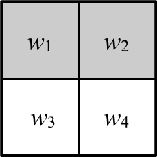 ◊ Let there be four equiprobable elementary events:
$\Omega =\{w_1,\,w_2,\,w_3,\,w_4\}.$
Consider three composite events $A=\{w_1,w_2\},$ $B=\{w_1,w_3\},$ $C=\{w_1,w_4\}$.
◊ Let there be four equiprobable elementary events:
$\Omega =\{w_1,\,w_2,\,w_3,\,w_4\}.$
Consider three composite events $A=\{w_1,w_2\},$ $B=\{w_1,w_3\},$ $C=\{w_1,w_4\}$.
Their probabilities are all $1/2$ (the shaded area in the image represents event $A$).
Since $A\,\&\,B~=~w_1$, then $P(A\,\&\,B) ~=~ P(w_1) ~=~1/4$, so:
$$
P(A,\,B)=P(A)\,P(B),~~~~~~~~
P(A,\,C)=P(A)\,P(C),~~~~~~~~
P(B,\,C)=P(B)\,P(C).
$$
However:
$$
P(A,\,B,\,C) = P(w_1) = \frac{1}{4} \neq P(A)\,P(B)\,P(C).
$$
Thus, from $A\Prep B$, $A\Prep C$, $B\Prep C$, it does not necessarily follow that $A\Prep B \Prep C$.
✒ It should also be noted that independence does not possess transitivity: $$ A\Prep B,~~B\Prep C~~~~~~\not\Rightarrow~~~~A\Prep C. $$ For example, this holds for such a joint probability: $P(A,B,C)=P(B)\,P(A,C)$.
✒ The requirement $P(X,Y,Z)=P(X)\,P(Y)\,P(Z)$ for the independence of three events $A\Prep B \Prep C$ includes all pairwise independencies if summing over the "unnecessary" event: $$ P(X,Y)~=~\sum_{Z}P(X,Y,Z) ~=~P(X,Y,z)+P(X,Y,\bar{z})~=~P(X)P(Y)\,\bigr(P(z)+P(\bar{z})\bigr)~=~P(X)P(Y), $$ since $P(z)+P(\bar{z})=1$, where $z$ is the event $Z$ occurred, and $\bar{z}$ is not occurred. Therefore, $A\Prep B \Prep C~~~\Rightarrow~~~A\Prep B$ and so on.
✒ Let's prove that the variance of the frequency of an event over $N$ trials is equal to $p_A(1-p_A)/N$. Consider experiments repeated many times, each consisting of $N$ trials observing event $A$. Let $X_i=1$, if event occurs in the $i$-th trial, otherwise $X_i=0$. This is a random variable, because in one experiment, in the $i$-th trial, the event may occur, and in another, it may not. The frequency of the event also becomes a random variable $P=(X_1+...+X_N)/N$ . Let's find its mean and variance over all experiments. If the "true" probability of the event is $p_A$, then for any $i$: $$ \langle X_i \rangle = 1\cdot p_A+0\cdot (1-p_A)=p_A,~~~~~~~~~~~~~~\langle X^2_i \rangle = 1^2\cdot p_A+0^2\cdot (1-p_A)=p_A. $$ Consequently, the average frequency is also $P_\text{ср}=\langle P \rangle = p_A$. Random variables $X_i$ and $X_j$ are independent (the event can occur in the trial independently of what happened in other trials). Therefore: $$ for~~i\neq j~~~~~~~~~~~\langle X_i\, X_j \rangle = \sum_{x_i, x_j} x_i \,x_j~ p(x_i,x_j) = \sum_{x_i, x_j} x_i\, x_j~ p(x_i)\,p(x_j) = \langle X_i \rangle\, \langle X_j \rangle, $$ where the sums go over the two values $0,1$ of each random variable. Now let's calculate the mean square of the frequency: $$ N^2\langle P^2 \rangle = \langle (X_1+...+X_N)^2 \rangle = \sum_i \langle X^2_i \rangle+ 2\sum_{i\lt j} \langle X_i X_j \rangle = \sum_i \langle X^2_i \rangle+ 2\sum_{i\lt j} \langle X_i \rangle \,\langle X_j \rangle = N p_A + N\,(N-1)\,p^2_A, $$ where it is taken into account that the first sum has $N$ identical terms, and the second has $N(N-1)/2$ terms. Now, using the formula $D=\langle P^2\rangle - P^2_\text{mean}$ we can easily find the variance $D=p_A(1-p_A)/N$.
Conditional independence
Two events $X,Y$ are called conditionally independent given event $Z$ if: $$ P(Z,\,Y\to X) = P(Z\to X),~~~~~~~~~~~~P(Z,\,X \to Y) = P(Z\to Y). $$ Conditional independence is similar to unconditional independence in the sense that the probability of occurrence of $X$ does not depend on whether event $Y$ occurred, and vice versa. However, these probabilities depend on a third event $Z$.
It is easy to verify that from this definition follows the relation $P(X,Y,Z)\,P(Z) = P(X,Z)\,P(Y,Z)$, which allows to factorize the joint conditional probability for conditionally independent $X,Y$: $$ P(Z\to X,\,Y) = P(Z\to X)\,P(Z\to Y). $$ Therefore, the independence of $X,Y$ given $Z$ is denoted as follows: $X\Prep Y\mid Z$.
In general, for the joint probability of three arbitrary events $X,Y,Z$ the chain rule holds: $P(X,Y,Z)=P(Z)\, P(Z\to X) \,P(Z,X\to Y).$ In the presence of conditional independence $X\Prep Y\mid Z$ the last factor is replaced by a simpler one: $$ P(X,Y,Z)=P(Z)\,P(Z\to X)\,P(Z\to Y). $$ Situations where $X_1\Prep X_2\Prep ...\Prep X_n\mid Z$ play an important role in machine learning. For example, $Z$ can be the presence of a disease, and $X_i$ - conditionally independent symptoms of it.
✒ It's worth checking that if $X,Y$ are conditionally independent and $X'$ is a subset of $X$, and $Y'$ is a subset of $Y$, then $X',Y'$ will also be conditionally independent: $$ X\Prep Y\mid Z,~~~~~X'\subseteq X,~~~~Y'\subseteq Y~~~~~~~\Rightarrow~~~~~~~X'\Prep Y'\mid Z $$ Recall that if $P(X'\to X)=1$, then $X' \subseteq X$ and $P(X',X)=P(X')$.
☝ Let's emphasize that from pairwise independence $X \Prep Y$ does not imply
conditional independence for $X \Prep Y \mid Z$, and vice versa - conditional independence, generally speaking,
does not imply unconditional pairwise independence.
Let's provide two examples.
 ◊ When $X:$ "a lot of ice cream is sold", and $Y$: "accidents happen in the water"
and $P(X,Y)\neq P(X)P(Y)$. But this is related to the presence of a third "controlling variable" - $Z$: "it's hot outside",
so people buy a lot of ice cream and swim in the water.
◊ When $X:$ "a lot of ice cream is sold", and $Y$: "accidents happen in the water"
and $P(X,Y)\neq P(X)P(Y)$. But this is related to the presence of a third "controlling variable" - $Z$: "it's hot outside",
so people buy a lot of ice cream and swim in the water.
In this case, it's likely that $X\Prep Y\mid Z$, but $X \NoPrep Y$ and
the joint probability is:
$$
P(X,Y,Z)~=~P(Z)\,P(Z\to X,Y)~=~P(Z)\,P(Z\to X)\,P(Z\to Y),
$$
where the first equality is the definition of conditional probability, and in the second $X\Prep Y\mid Z$ is taken into account.
 ◊ Let's consider the scenario of rolling two dice. The outcomes of the dice rolls, denoted as $X,Y$ are independent $X\Prep Y$.
However, if we have information $Z$: "the sum of the scores is divisible by 6",
then the events are not conditionally independent. $Z$ occurs when
$\{(X,\,Y)\} = \{(1,\,5);\, (5,\,1);\, (2,\,4);\, (4,\,2);\, (3,\,3);\, (6,\,6)\}$,
hence $P(Z\to X=3,Y=3)=1/6$. At the same time $P(Z\to X=3)=P(Z\to Y=3)~=~1/6$,
so there is no conditional independence: $1/6 \neq (1/6)(1/6)$.
◊ Let's consider the scenario of rolling two dice. The outcomes of the dice rolls, denoted as $X,Y$ are independent $X\Prep Y$.
However, if we have information $Z$: "the sum of the scores is divisible by 6",
then the events are not conditionally independent. $Z$ occurs when
$\{(X,\,Y)\} = \{(1,\,5);\, (5,\,1);\, (2,\,4);\, (4,\,2);\, (3,\,3);\, (6,\,6)\}$,
hence $P(Z\to X=3,Y=3)=1/6$. At the same time $P(Z\to X=3)=P(Z\to Y=3)~=~1/6$,
so there is no conditional independence: $1/6 \neq (1/6)(1/6)$.
The diagrams shown on the right are called Bayesian networks. They play an important role in machine learning and probabilistic logical inference theory. Probabilistic reasoning or inference involves constructing a probabilistic model $P(X_1,...,X_n)$ for $n$ variables (random variables). Typically, only a subset of variables is known. Based on this information, one needs to determine the probabilities of other variables, for example: $P(X_1,X_2\to X_3)$. The main problem lies in constructing the probabilistic model. Even for binary random variables (=events), specifying $2^n-1$ numbers is required. This is computationally challenging for large $n$ and unrealistic empirically. In this situation, conditional independencies between variables come to the rescue, allowing the joint probability to be decomposed into the product of simpler ones.
