ML: Bayesian Methods
Introduction
Bayes' formula plays a crucial role in machine learning and artificial intelligence algorithms. This document is a continuation of the introduction to probability theory and is dedicated to various aspects of applying this formula..
Bayes' formula
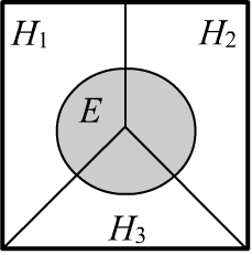
Let there be $n$ mutually exclusive (non-overlapping) events $\{H_1,...,H_n\}$, $H_i\,\cap\,H_j=\varnothing$, which will be referred to as hypotheses. One of them is assumed to be true (necessarily occurs in a trial): $$ \sum_i P(H_i) = 1. $$ In the simplest case, there may be two incompatible hypotheses, concerning whether a certain statement $D$ is either true or false:
We assume that the probabilities of the hypotheses $P(H_i)$ are known. They can be obtained from observations (above, this is the proportion of the population that is sick - objectivist interpretation) or or they can be the degree of "confidence" or "belief" in the truth of the hypothesis by the decision-maker (subjectivist interpretation). These probabilities are called prior probabilities ("before experience", Latin "a priori").
When some event $E$ occurs (providing new information),
it may change the probabilities of the hypotheses into posterior probabilities $P(E\to H_i)$
(obtained from experience, Latin. "a posteriori").
They are determined by Bayes' formula:
$$
P(E\to H_i) ~=~ \frac{P(E,H_i)}{P(E)} ~=~ \frac{P(H_i)\,P(H_i\to E)}{P(E)}.
$$
 The probability of the event $P(E)$ for complete (covering all cases) and inconsistent hypotheses
is calculated using the law of total probability:
$$
~~~~~~~~~~~~~~~~~~~~~~~~~~~~~~~P(E) ~=~ \sum_j P(H_j)\,P(H_j\to E) ~=~ \sum_j P(E,\,H_j).
$$
As a result, the sum of $P(E\to H_i)$ across all $H_i$ is equal to one
(one of the hypotheses is true).
The probability of the event $P(E)$ for complete (covering all cases) and inconsistent hypotheses
is calculated using the law of total probability:
$$
~~~~~~~~~~~~~~~~~~~~~~~~~~~~~~~P(E) ~=~ \sum_j P(H_j)\,P(H_j\to E) ~=~ \sum_j P(E,\,H_j).
$$
As a result, the sum of $P(E\to H_i)$ across all $H_i$ is equal to one
(one of the hypotheses is true).
According to Bayes' formula, the posterior probability $P(E\to H_i)$ is proportional to the prior probability $P(H_i)$, multiplied by the "likelihood function" $P(H_i\to E)$ of event $E$ given hypothesis $H_i$. In particular, if the probability of the event does not depend on the truth of the hypothesis $P(H_i\to E)=P(E)$, then the prior probability remains unchanged: $P(E\to H_i)=P(H_i)$.
It is often easier to gather statistics to calculate the probabilities $P(H_i\to E)$ than for $P(E\to H_i)$. For example, in the case of $H:$ "the person is sick with a certain disease", you can take a group of sick people and calculate the probability $P(H\to E)$ for symptom $E$. At the same time, symptom $E$ may arise due to a variety of different causes (diseases) unrelated to disease $H$.
Additionally, the probabilities $P(H\to E)$ are often more stable than $P(E\to H)$. For example, in the case of an epidemic, the probability $P(H)$ increases, but $P(H\to E)$ remains unchanged. According to Bayes' formula, $P(E\to H)$, will, of course, also increase.
Example: Disease testing
| $p$ | ${n}$ | Tot | |
|---|---|---|---|
| $d$ | 9 | 1 | 10 |
| $\bar{d}$ | 90 | 9900 | 9990 |
| Tot | 99 | 9901 | 10000 |
Instead of talking about events, let’s refer to random variables that take on two values:
Hypothesis $H=\{d,\bar{d}\}$, where
$d$ - "the person has disease $D$" and
$\bar{d}$ - "the person does not have this disease";
Event $~E=\{p,n\}$, where $p$ - test is positive, and $n$ - test is negative:
$$
P(d\to p) = 0.9,~~~~~~~P(\bar{d}\to p) = 0.009,~~~~~~P(d) = 0.001.
$$
On the right in the table is the data (in people) from which these probabilities were estimated.
The values of $P(H\to E)$ are calculated by rows, and $P(E\to H)$ - by columns: $P(d\to p)=9/10$, $P(p \to \bar{d})=90/99$.
The probability of getting a positive test (regardless of the person’s condition) is: $$ P(p ) = P(d)\,P(d\to p ) ~+~ P(\bar{d})\,P(\bar{d}\to p ) = 0.9*0.001 + 0.009*(1-0.001)= 0.0099 $$ Naturally, the same value can be obtained from the table (tot in the first column 99/10000).
According to Bayes' formula, the posterior probability of being sick is: $$ P(p \to d) = \frac{P(d)\,P(d\to p )}{P( p )} = \frac{0.001\cdot 0.9}{0.00989} = 0.091. $$ This result is also derived from the first column of the table: 9/99.
It is curious that, although the test works fairly accurately for healthy people (failing $9$ times out of $1000$ tests), the probability of being sick after a single positive test is only $9\%$. This seemingly paradoxical result is due to the fact that, although the test makes few errors, the proportion of sick people in the overall population is even smaller. It’s worth analyzing the table given above (if the test were conducted across the entire population, there would be 99 people with positive results, but only 9 of them would actually be sick).
☝ It is often more convenient to normalize the posterior probabilities of the hypotheses at the end, omitting the common factors that do not depend on the hypotheses during calculations. For the testing example, it would look like this (the symbol $\sim$ indicates that the values are proportional, i.e., equal up to a common factor that does not depend on $d$, $\bar{d}$): $$ \begin{array}{lclcl} P( p \to d) &\sim& P(d) \, P(d\to p ) &=& 0.9\cdot 0.001, \\ P( p \to \bar{d}) &\sim& P(\bar{d})\, P(\bar{d}\to p ) &=& 0.009\cdot 0.999. \end{array} $$ We express $P( p \to H)$ as a vector, whose components correspond to $H=d$ and $H=\bar{d}$: $$ P( p \to H) ~\sim~ \bigr\{ 0.9\cdot 0.001,~~~~ 0.009\cdot 0.999\bigr\} ~\sim~ \bigr\{ 0.1,~~~~ 0.999\bigr\}, $$ where common factors have been factored out and omitted. Now the vector needs to be normalized to one: $P( p \to H)=\bigr\{ 0.1,~~~~ 0.999\bigr\}/(0.1+0.999)=\bigr\{ 0.091,~~~~ 0.909\bigr\} $.
Sequence of observations
When making decisions, Bayes' formula is used to update probabilities as new information becomes available. Suppose two independent tests were conducted (either sequentially or simultaneously, but in different laboratories). What will the posterior probabilities be in this case?
Let $E_1$ and $E_2$ represent two conditionally independent events (for example, "pp" or "pn"). The probability of the hypothesis $H_i$ being true after these events occur, according to Bayes' formula, is (considering $\{E_1,\,E_2\}$ as one event): $$ P(E_1,E_2 \to H_i) = \frac{P(H_i)\,P( H_i\to E_1,E_2 )}{P(E_1,E_2)} = \frac{P(H_i)\,P(H_i\to E_1)\,P(H_i\to E_2)}{P(E_1,E_2)}. $$ In the second equality, it is taken into account that events $E_1$ and $E_2$ are conditionally independent (given hypothesis $H_i$). The probability in the denominator, as before, is found from the normalization condition for $P(E_1,E_2 \to H_i)$: $$ P(E_1,E_2) ~=~ \sum_j P(H_j)\,P(H_j\to E_1)\,P(H_j\to E_2). $$
Note that although the tests are conditionally independent, they are not unconditionally independent: $P(E_1,E_2) \neq P(E_1)\,P(E_2)$, Why does this happen?
Answer
This is easier to understand in the context of disease testing. The relation $P(E_1,E_2) = P(E_1)\,P(E_2)$ would hold if the test results $E_1$ and $E_2$ were obtained from two randomly selected people. In our case, the test is conducted on the same person who is either sick or healthy. We don't know which hypothesis is true, but one of them must be. Therefore, $P(E_1,E_2) ~=~ P(h)\,P( h\to E_1,E_2)+P(\bar{h})\,P(\bar{h}\to E_1,E_2 )$.The formula for the posterior probability can be rewritten as follows: $$ P(E_1\to H_i) = \frac{P(H_i)\,P(H_i\to E_1 )}{P(E_1)},~~~~~~~~~~~~~~ P(E_1,E_2 \to H_i) = \frac{P(E_1\to H_i)\,P(H_i \to E_2)}{P(E_1\to E_2)}. $$ Thus, event $E_1$ updates the prior probability $P(H_1)$ to $P(E\to H_1)$, which is then further refined (using the same Bayes' formula) into an even more precise probability of the hypothesis $P(E_1,E_2\to H_i)$, and so on. The sequence of conditionally independent events does not affect the outcome.
Example of calculations on numpy
Here is an example of calculating disease testing probabilities using Python with the help of the NumPy library:import numpy as np np.set_printoptions(precision=5, suppress=True)We will start joint probabilities with the prefix P_, and conditional probabilities with C_.
The numbering of events: E=[p,n] and hypotheses: H=[sick, healthy]. The initial data is as follows:
NH, NE = 2, 2                          # number of hypotheses and events

P_H  = np.array([0.001, 1-0.001])      # [P(sick), P(healthy)]

C_EH = np.array([[  0.9,   0.009],     # P(sick -> p) P(healthy -> p)
                 [1-0.9, 1-0.009] ])   # P(sick -> n) P(healthy -> n)
Results for a single test:
C_HE = ( C_EH*P_H.reshape(1,NH) ).T    # [[P(p -> sick), P(n -> sick)],      [[0.09099 0.0001]
C_HE /= C_HE.sum(0)                    #  [P(p -> healthy), P(n -> healthy)]]   =   [0.90901 0.9999]]
Results for two tests:
C_HEE = (C_EH.reshape(NE,1,NH)*C_EH.reshape(1,NE,NH)*P_H.reshape(1,1,NH)).transpose(2,0,1)
C_HEE /= C_HEE.sum(0)

# P(pp -> sick)  P(pn -> sick)  [[[0.90917 0.01   ]
# P(np -> sick)  P(nn -> sick)    [0.01    0.00001]]
#
# P(pp -> healthy)  P(pn -> healthy)   [[0.09083 0.99   ]
# P(np -> healthy)  P(nn -> healthy)    [0.99    0.99999]]]
Thus, the probability of being sick with two positive tests $P(pp\to \text{sick})=0.909$ is significantly higher than with just one test: $P(p\to \text{sick})=0.091$.
Classification problem
In a classification problem with non-overlapping classes, an object with features $\mathbf{x}=\{x_1,...,x_n\}$ needs to be assigned to one of $C$ classes. Let $P(\mathbf{x} \to c)$ represent the conditional probability that an object with features $\mathbf{x}$ belongs to class $c$, where $c\in [0...C-1]$. Then, Bayes' theorem can be written as follows: $$ P(\mathbf{x} \to c) ~=~ \frac{p(c,\mathbf{x})}{p(\mathbf{x})} = \frac{P(c)\,p(c\to \mathbf{x})}{p(\mathbf{x})}, ~~~~~~~~~~~~~ p(\mathbf{x}) ~=~ \sum_\alpha P(\alpha)\,p(\alpha\to \mathbf{x}), $$ where $P(c)$ is the probability of a randomly chosen object belonging to class $c$ (regardless of its feature values), and $p(c\to \mathbf{x}) = p(c,\mathbf{x})/P(c)$ is the probability density function of the feature values $\mathbf{x}$ for objects from class $c$. The normalization in the denominator $p(\mathbf{x})$ is the distribution of objects in the feature space. If there are $N$ objects, then $p(\mathbf{x})\cdot N$ is the density of the number of objects per unit volume.
Thus, to obtain the probability $P(\mathbf{x}\to c)$, it is necessary to know the class probabilities $P(c)$ and the probability density function $p(c\to \mathbf{x})$. If the training set is unbiased (the classes are represented with the same frequency as in the test set), then $P(c)$ is easy to obtain. However, finding $p(c\to \mathbf{x})$ in a multidimensional feature space is often challenging. If the objects in a class form compact "clusters," $p(c\to \mathbf{x})$ can be approximated with smooth functions (e.g., multivariate Gaussian distributions). The parameters of these functions are obtained from a set of training examples. Another approach is to find the nearest neighbors to point $\mathbf{x}$ in each class and use them to construct approximating surfaces $p(c\to \mathbf{x})$.
Sometimes, good results can be achieved using naive Bayes, which assumes conditional independence of the features: $$ p(c\to \mathbf{x}) ~=~p(c\to x_1)\cdot...\cdot p(c\to x_n). $$ The probabilities $p(c\to x_i)$ are especially easy to calculate for categorical or binary features. In this case, such a classifier may be more effective than metric models. If the features are continuous, then for $p(c\to x_i)$, one can build histograms or compute statistics from the training data (for example, when assuming that $p(c\to x_i)$ follows a normal distribution).
When using naive Bayes, two problems may arise — loss of precision
when multiplying small numbers and zero probabilities for some $p(c\to x_i)$
(if there is little training data).
The first problem is addressed by switching to logarithms (instead of the product there will be a sum).
To handle zero probabilities Laplace smoothing is applied.
Part-of-speech tagging
Bayes' theorem can be used to assign each word $w_i$ in a sentence its part of speech $t_i$: noun (N), adjective (A), verb (V), etc. (this is known as Part-of-Speech Tagging). Let $t_i$ represent one of the tags (N, A, V...). If the conditional probability $P(w_1,...,w_n\to t_1,...,t_n)$ is known for the words $w_1...w_n$ in the text, the task is solved by finding the maximum of this probability: $$ t_1,...,t_n = \arg\max_{t_1,...,t_n}\,P(w_1...w_n\to t_1...t_n). $$ To estimate the probability, we apply Bayes' theorem: $$ P(w_1...w_n\to t_1...t_n) ~=~ \frac{P(w_1...w_n,t_1...t_n)}{P(w_1...w_n)} ~=~ \frac{P(t_1...t_n)\,P( t_1...t_n \to w_1...w_n)}{P(w_1...w_n)} $$ To maximize on $t_i$, only the numerator needs to be considered. The probability $P(t_1...t_n)$ characterizes the likelihood of a given sequence of parts of speech (e.g., N V is more likely than A V). As a first approximation, bigrams can be used to estimate this. In this case, the Markov simplification is applied using the chain rule: $P(t_1...t_{k-1}\to t_k)=P(t_{k-1}\to t_k)$: $$ P( t_1...t_n) = P(t_1)\cdot P(t_1\to t_2)\cdot... \cdot P(t_{n-1}\to t_n). $$ The second probability is estimated in the simplest case using such bigrams: $$ P( t_1...t_n \to w_1...w_n) ~=~ P( t_1...t_n \to w_1)\cdot ... \cdot P( t_1...t_n \to w_1) ~=~ P(t_1\to w_1)\cdot...\cdot P(t_n\to w_n). $$ This assumes (rather roughly) conditional independence of words in the sequence. Note that, by the same Bayes' theorem, $P(t\to w)=P(w\to t)\,P(w)/P(t)$.Guess what was intended
Intelligent systems designed to determine a person's intentions are quite common. These systems ask a series of questions, to which the person responds with Yes or No. A well-known example is the game Akinator, which guesses the character a person is thinking of.
Let’s assume the person has thought of one of the objects $X=\{x_1,...,x_N\}$. The system asks a question $Q_i\Rightarrow \{y_i, n_i\}$, to which it receives a binary response $y_i$ (yes) or $n_i$ (no). For example: "Is your character a woman?", "Is your character from real life?", "Is your character friends with the bear?", etc. When building such a system, it’s important to consider that a person may intentionally or accidentally give incorrect answers. Therefore, in general, both conditional probabilities: $P(X\to y_i)$ and $P(X\to n_i)$ are non-zero — meaning the system can receive a $y_i$ or $n_i$ response to question $Q_i$ when the object is from the set $X$.
| yes | $y_1$ | $y_2$ | ... | $y_M$ | $P(x)$ |
|---|---|---|---|---|---|
| $x_1$ | 9 | 1 | ... | 2 | 0.001 |
| $x_2$ | 10 | 0 | ... | 25 | 0.008 |
| ... | ... | ... | ... | ... | ... |
| $x_N$ | 0 | 890 | ... | 100 | 0.02 |
Let’s denote by $I_k$ the sequence of $k$ question-answer pairs obtained by the system:
$I_k=\{Q_1,...,Q_k\}$.
Based on this information, conditional probabilities $P(I_k\to X)$ are formed for each object in $X$.
Using Bayes' theorem, we can write:
$$
P(I_k\to X) = \frac{P(X)\,P(X\to I_k)}{P(I_k)} = \frac{P(X)\,P(X\to Q_1)...P(X\to Q_k)}{P(I_k)},
$$
where in the second equation, the assumption (a relatively rough one) is made that question-answer pairs do not influence each other.
The normalization probability $P(I_k)$, as usual, is found from the normalization condition (sum over all $x_i$),
assuming the person has thought of an object known to the system.
Since the task is to find $x$ with the maximum value of $P(I_k\to X)$, the denominator can be omitted:
$$
x= \text{arg}\max_X ~\,P(X)\,P(X\to Q_1)...P(X\to Q_k).
$$
The choice of the next question $Q$ after a series of question-answer pairs $I_{k-1}$ is made similarly to the ID3 algorithm for building decision trees. The only difference is that the "feature" $Q$ can have two values $\{y,n\}$. The optimal question is the one that makes the distribution of probabilities $P=P(I_{k-1},\, Q_k\to X)$ as uneven as possible (increases the probabilities of certain objects). The entropy $H[P]$ of this distribution should be minimal (we average the entropies for "yes" and "no" answers): $$ Q = \text{arg}\min_{Q}~ H[ P(I_{k-1},\, y\to X)]\,P(y) + H[ P(I_{k-1},\, n\to X)]\,P(n), $$ where the probabilities $P(Q)$ are calculated taking into account the known probability of the object $x$ at this point: $$ P(Q) = \sum_{x} P(X\to Q)\,P(I_{k-1}\to X). $$
Estimation of model parameters
It is often necessary to estimate some parameter, for example, a continuous parameter $\theta$, based on an available observation $x$. Usually, $\theta$ is a statistical parameter (event probability, distribution parameters, etc.).
Let’s assume the prior probability distribution $p(\theta)$ of the parameter $\theta$ is known. In the complete absence of information about its value, the distribution is uniform $p(\theta)=\text{const}$. If there have been previous observations or subjective considerations, the distribution function $p(\theta)$ may be more defined.
The posterior distribution of the parameter (after observation $x$) is calculated, as usual, using Bayes' theorem: $$ p(x\to \theta) ~=~ \frac{p(\theta)\,p(\theta\to x)}{p(x)},~~~~~~~~~~~~~~~p(x) ~=~ \int p(\theta)\,p(\theta\to x)\,d\theta, $$ where the integration is carried out over the entire range of "allowed" values of $\theta$. To compute $p(x\to \theta)$, besides the prior distribution $p(\theta)$, the likelihood function $p(\theta\to x)$ must also be known, which is usually specified based on theoretical considerations.
When the parameter $\theta$ is a multidimensional vector $\{\theta_1,...,\theta_n\}$, calculating the $n$-dimensional integral with the required accuracy can be challenging. To avoid such difficulties, $p(\theta)$ is chosen in a way that the integral can not only be computed analytically, but the resulting posterior distribution $p(x\to \theta)$ also leads to analytical results with further observations.
◊ Consider determining the probability of an event based on observing
whether it occurred or not.
In this case, $x=1$ (the event occurred in the observation) and $x=0$ (it did not occur).
We choose the Bernoulli distribution as the prior:
$$
p(\theta) = \frac{\theta^{\alpha-1}\,(1-\theta)^{\beta-1}}{\mathrm{B}(\alpha,\beta)}.
$$
The real-valued parameters $\alpha and \beta$ are hyperparameters,
and their assignment results in different forms of the distribution $p(\theta)$.
For example, $\alpha=\beta=1$ gives a uniform distribution.
When $\alpha=\beta=10$, the distribution has a symmetric peak
around $\theta=0.5$, and so on.
The normalization factor $\mathrm{B}(\alpha,\beta)$ is the beta function, expressed through gamma functions:
$$
\mathrm{B}(\alpha,\beta) = \int\limits_0^1 t^{\alpha-1}(1 - t)^{\beta-1}\,dt = \frac{\Gamma(\alpha) \Gamma(\beta)}{\Gamma(\alpha+\beta)}.
$$
If the event is random and occurs with a stable frequency, the probability that it will or will not occur is given by: $$ p(\theta\to x) = \left\{ \begin{array}{lll} \theta & x=1\\ 1-\theta & x=0 \end{array} \right. $$
In general, after $n+m$ observations, where the event occurred $n$ times and did not occur $m$ times, the posterior probability is: $$ P(n,m\to \theta) = \frac{x^{n+\alpha-1}\,(1-x)^{m+\beta-1}}{\text{B}(n+\alpha,\,m+\beta)}. $$ Depending on the values of the hyperparameters $\alpha and \beta$ and the results of observations, various distributions for the probability $\theta$ are obtained.
