ML: Introduction to Machine Learning
Introduction
 Machine learning methods are a subset of artificial intelligence algorithms.
In turn, neural networks and deep learning are special cases of machine learning.
This document is introductory and describes the basic concepts of machine learning and the types of problems
it helps solve.
Machine learning methods are a subset of artificial intelligence algorithms.
In turn, neural networks and deep learning are special cases of machine learning.
This document is introductory and describes the basic concepts of machine learning and the types of problems
it helps solve.
Objects and their features
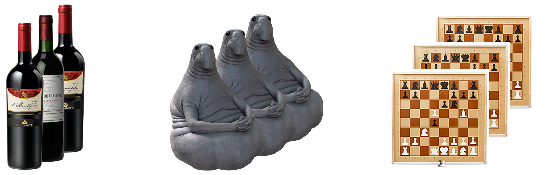 Let's consider a set of similar objects:
wine bottles, hospital visitors, or positions on a chessboard (these are three different sets).
Each object in the set is characterized by a set (vector) of features:
$\mathbf{x}= \{x_0,x_1,...,x_{n-1}\}$.
Let's consider a set of similar objects:
wine bottles, hospital visitors, or positions on a chessboard (these are three different sets).
Each object in the set is characterized by a set (vector) of features:
$\mathbf{x}= \{x_0,x_1,...,x_{n-1}\}$.
Features can be:
- Numeric (weight, height, pixel brightness)
- Binary (female/male, alive/dead)
- Ordered non-numeric (small/large/huge)
- Qualitative non-numeric (red/blue/green)
Machine learning tasks
Objects in this set can sometimes be divided into classes (e.g., a person: {healthy, sick}, wine: {Italian, French, Georgian}). Additionally, each object can be associated with a number y (e.g., the degree of white's advantage in a chess position; the quality of wine according to experts' average opinion). Accordingly, two tasks are often solved: classification - determining which class the object belongs to and regression - determining which number or set of numbers corresponds to the object. For example:
- 1) 3 feature: x={temperature,hemoglobin,cholesterol}; 2 classes: {0: healthy, 1: sick};
- 2) w*h features: x={brightness of pixels in an image of size w times h}; 10 classes: {0-9: digit in the image}.
- 3) 8*8*13 features: x={codes of chess pieces}; regression: white's advantage over black =[-1...1].
For successful classification or regression tasks, the features characterizing the object must be significant, and the feature vector must be complete (sufficient for classifying objects or determining the regression value y).
Besides classification and regression, other tasks are possible. For example, in ranking, it is required to order a set of objects according to some criterion (e.g., documents retrieved by a search query). Recently, generative tasks have played an important role: generating another sequence of objects from a given ordered sequence of objects from the same or different set. Examples include machine translation systems, image captioning, or generating fake videos.
Supervised learning
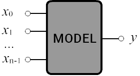
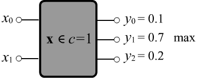
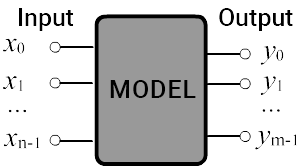 Let's represent a system solving a classification or regression task as a black box.
It has n inputs where feature values
$\mathbf{x} = \{x_0,...,x_{n-1}\}$
are fed and $m$ outputs $\mathbf{y} = \{y_0,...,y_{m-1}\}$.
In a classification task $m$ is equal to the number of classes, while in a regression task,
it equals the number of dependent values associated with each object.
The model can be considered a multidimensional function or algorithm $\mathbf{y}=f(\mathbf{x},\,\boldsymbol{\omega})$,
that outputs $\mathbf{y}$ given $\mathbf{x}$.
The vector $\boldsymbol{\omega}$ - are the model parameters.
Let's represent a system solving a classification or regression task as a black box.
It has n inputs where feature values
$\mathbf{x} = \{x_0,...,x_{n-1}\}$
are fed and $m$ outputs $\mathbf{y} = \{y_0,...,y_{m-1}\}$.
In a classification task $m$ is equal to the number of classes, while in a regression task,
it equals the number of dependent values associated with each object.
The model can be considered a multidimensional function or algorithm $\mathbf{y}=f(\mathbf{x},\,\boldsymbol{\omega})$,
that outputs $\mathbf{y}$ given $\mathbf{x}$.
The vector $\boldsymbol{\omega}$ - are the model parameters.
Machine learning implies the presence of a training set of objects $\mathcal{T}$. It is provided by a "teacher" (usually a human). The system learns on this set (configures the model = optimizes the parameters $\boldsymbol{\omega}$). A properly trained system should produce correct results not only on the training set but also on a test set of objects $\mathcal{V}$, that were not used in training: $\mathcal{T}\cap \mathcal{V}=\varnothing$.
Two common problems in machine learning are under-fitting
and over-fitting.
Underfitting occurs when the model is too simple and cannot express the nature of the training data,
for example, due to insufficient "tunable" parameters.
Overfitting is the opposite situation: the model has too many parameters and tries
to "remember" all the training objects, including inevitable noise or errors.
In this case, the model cannot generalize or extrapolate and performs poorly
on test data.
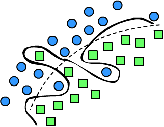 On the right is an illustration of a two-class classification problem (circles and squares)
in a two-dimensional feature space. The dotted line is a smooth separating surface,
that distinguishes objects of one class from those of another. Three objects are misclassified by this surface.
This situation is "corrected" by the wavy line. However, if these three objects are random outliers,
the wavy line is a typical example of overfitting.
On the right is an illustration of a two-class classification problem (circles and squares)
in a two-dimensional feature space. The dotted line is a smooth separating surface,
that distinguishes objects of one class from those of another. Three objects are misclassified by this surface.
This situation is "corrected" by the wavy line. However, if these three objects are random outliers,
the wavy line is a typical example of overfitting.
Mean squared error
Consider $N$ objects characterized by $n$-dimensional feature vectors. They can be represented as a matrix $x_{i\alpha}$, where the first index $i=0...N-1$ - is the object number, and the second index $\alpha=0...n-1$ - is the feature number. For each ($i$-th) example $\hat{\mathbf{x}}_i=\{\hat{x}_{i0},...,\hat{x}_{i,n-1}\}$ from the training set, the "true" values of the model outputs (e.g., in a regression task) are known. These will be marked with a hat: $\hat{\mathbf{y}}_i=\{\hat{y}_{i0},...,\hat{y}_{i,m-1}\}$. The closer $\mathbf{y}=f(\hat{\mathbf{x}},\,\boldsymbol{\omega})$ to the true values $\hat{\mathbf{y}}$, the better the model works.
The mean squared error (MSE) is defined as the average of the squares of deviations of the model predictions $y_{i\alpha}$ from the true values $\hat{y}_{i\alpha}$ for each example ($i$) and each output ($\alpha$):
$$ L = \langle(\mathbf{y}-\hat{\mathbf{y}})^2 \rangle ~=~ \frac{1}{N\cdot m}\sum^{N-1}_{i=0}~\sum^{m-1}_{\alpha=0} ~~(y_{i\alpha}-\hat{y}_{i\alpha})^2. $$ Since the model $\mathbf{y} = f(\hat{\mathbf{x}}, \boldsymbol{\omega})$ and the training set $\{\hat{\mathbf{x}},\hat{\mathbf{y}}\}$ are given, the error depends only on the model parameters $L=L(\boldsymbol{\omega})$. During machine learning, these parameters are adjusted to minimize the error: $\bar{\boldsymbol{\omega}} = \text{argmin} \,L(\boldsymbol{\omega})$.
A significant advantage of MSE is its differentiability with respect to the model outputs $\mathbf{y}$, and consequently, with respect to its parameters (if the function $f$ is differentiable): $$ \frac{\partial L}{\partial \boldsymbol{\omega}} ~=~ \sum_{i,\alpha} \frac{\partial L}{\partial y_{i\alpha}} \frac{\partial y_{i\alpha}}{\partial \boldsymbol{\omega}} ~=~ \frac{2}{N\cdot m}\sum_{i,\alpha} ~~(y_{i\alpha}-\hat{y}_{i\alpha})\,\frac{\partial f_{i\alpha}(\hat{\mathbf{x}}_i,\,\boldsymbol{\omega})}{\partial \boldsymbol{\omega}}. $$ This property of the mean squared error allows using the powerful optimization method of gradient descent for adjusting the model parameters.
Binary classification
 In the task of binary classification, an object with features $\mathbf{x}$
needs to be assigned to one of two classes: $c\in \{0,1\}$.
We assume the model has a single output $y$
with values in the range [0...1].
Then the classification rule is written as: $c = [y > 0.5]$.
Square brackets around the logical [condition] mean the number 0
if the condition is false and 1 if it is true.
Thus, if the model output is less than or equal to 0.5 we consider it as class $c=0$,
otherwise, it is class $c=1$.
In the task of binary classification, an object with features $\mathbf{x}$
needs to be assigned to one of two classes: $c\in \{0,1\}$.
We assume the model has a single output $y$
with values in the range [0...1].
Then the classification rule is written as: $c = [y > 0.5]$.
Square brackets around the logical [condition] mean the number 0
if the condition is false and 1 if it is true.
Thus, if the model output is less than or equal to 0.5 we consider it as class $c=0$,
otherwise, it is class $c=1$.
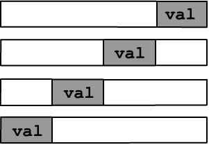
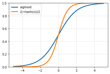 ☝ Scaling the model output to the interval $[0...1]$ can always be done using the sigmoid function:
$$
y = \sigma(x) = \frac{1}{1+e^{-x}},~~~~~~~~~~~\frac{dy}{dx} = y\cdot(1-y).
$$
For large $x$ the sigmoid quickly approaches one, for large negative values, it approaches zero, and $\sigma(0)=1/2$.
Alternatively, the hyperbolic tangent can be used: $y=(1+\tanh(x))/2$ with similar properties.
☝ Scaling the model output to the interval $[0...1]$ can always be done using the sigmoid function:
$$
y = \sigma(x) = \frac{1}{1+e^{-x}},~~~~~~~~~~~\frac{dy}{dx} = y\cdot(1-y).
$$
For large $x$ the sigmoid quickly approaches one, for large negative values, it approaches zero, and $\sigma(0)=1/2$.
Alternatively, the hyperbolic tangent can be used: $y=(1+\tanh(x))/2$ with similar properties.
The model error (which is minimized) can be taken as the mean squared error MSE, assuming that in the training set for the first class $\hat{y}_i = 0$, and for the second one: $\hat{y}_i = 1$: $$ L = \frac{1}{N}\sum_{i} (y_i - \hat{y}_i)^2 ~=~ \frac{1}{N}\sum_{i} \left\{ \begin{array}{cl} y^2_i, & \hat{y}_i =0\\ (1-y_i)^2, & \hat{y}_i = 1 \end{array} \right\}. $$ The closer the model's output is to zero or one, the more "confident" it is, and when $y\sim 0.5$ the model "doesn't know" to which class the object should be assigned.
Since the model output $y$ of $f(\mathbf{x},\,\boldsymbol{\omega})$ lies in the interval [0...1], it can be interpreted as the conditional "probability" $y=p(c=1|\mathbf{x})$ of the object $\mathbf{x}$ belonging to class $c=1$. Correspondingly, $1-y = p(c=0|\mathbf{x})$ - is the probability of belonging to class $c=0$. If $\hat{y}=1$, then it is necessary to maximize the probability $y$, and if $\hat{y}=0$, then to maximize the probability $1-y$. The maximum probability corresponds to the minimum of its negative logarithm. As a result, we get the following alternative to MSE: $$ L = -\frac{1}{N}\sum_{i} \Bigr[ \hat{y}_i \,\log y_i + (1-\hat{y}_i)\,\log(1-y_i) \Bigr] ~=~ -\frac{1}{N}\sum_{i} \left\{ \begin{array}{cl} \log (1-y_i), & \hat{y}_i =0\\ \log y_i, & \hat{y}_i = 1 \end{array} \right\}, $$ which is called binary cross-entropy (BCE). Below are the graphs of $L(y)$ for MSE and BSE at $\hat{y}=0$ and $\hat{y}=1$:
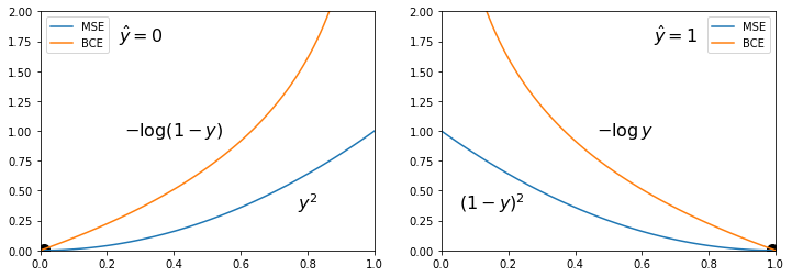
BСE approaches the target value $y=\hat{y}$ more steeply than MSE and is linear in the vicinity of the target value. This is why BCE is more popular for binary classification tasks.
Model accuracy
The errors introduced above are convenient for finding optimal parameters (e.g., using the gradient method). However, for practical purposes, additional quality assessments of the model that are easier to interpret are necessary. This is especially relevant for classification tasks. For binary classification, the simplest and most natural measure is the model accuracy, which is the proportion of correctly predicted classes: $$ A =\frac{\text{correct}}{\text{total}} = \frac{1}{N}\sum_i \bigr[ [y_i > 0.5 ] = \hat{y}_i \bigr] $$ If $A=1$, it means that the model correctly classifies all objects. If $A=0.5$, it performs no better than a random number generator.
Let's give an example of calculating the errors and model accuracy using the NumPy library:
import numpy as np                                         # Importing the numpy library

y = np.array([0.1, 0.8, 0.6, 0.2])                         # Outputs for 4 examples
c = np.array([0,   1,   0,    0])                          # Their true classes

mse = np.mean( (y-c)**2 )                                  # Mean Squared Error
bce = np.mean( -c*np.log(y)-(1-c)*np.log(1-y) )            # Binary Cross-Entropy
acc = np.mean( (y > 0.5) == c )                            # Model Accuracy

print(f'mse:{mse:0.2f}, bce:{bce:0.2f}, acc:{acc:0.2f}')   # mse:0.11, bce:0.37, acc:0.75
In the array "y" are the model outputs for four examples,
and in the array "с" are the corresponding "true" classes (binary classification).
In the worst-case scenario, when the model is always unsure (outputs 0.5 for any $\mathbf{x}$), the errors are: mse=0.25 and bce=0.69, i.e., bce is greater than mse, but both are zero at the minimum point (see the diagram above).
Positive and negative class
The accuracy criterion makes sense when the number of objects in each class is roughly equal. However, often one type of object is more frequent than the other. A model that always predicts the more frequent class will have a decent accuracy (equal to the frequency of that class), but in fact, it has not learned anything meaningful.
In medical diagnostics, the terms positive
and negative are used.
Test results are negative if no pathology (disease)
is detected, and positive if it is detected.
Accordingly, for a randomly chosen person, the probability of negative results is significantly higher
than positive results. Therefore, in binary classification with a noticeable class frequency imbalance,
the more likely class is called negative, and the less likely one is called positive.
Let's draw a set of objects. On the left side of the vertical dotted line are the objects of the negative class, and on the right are the positive ones. The bold wavy line separates the negative and positive classes from the model's perspective. In doing so, it makes two types of errors:
- False positive (FP) - objects of the negative class are classified
as positive
(healthy individuals are considered sick), shown in yellow below; - False negative (FN) - objects of the positive class
are classified as negative
(sick individuals are not detected), shown in green below.
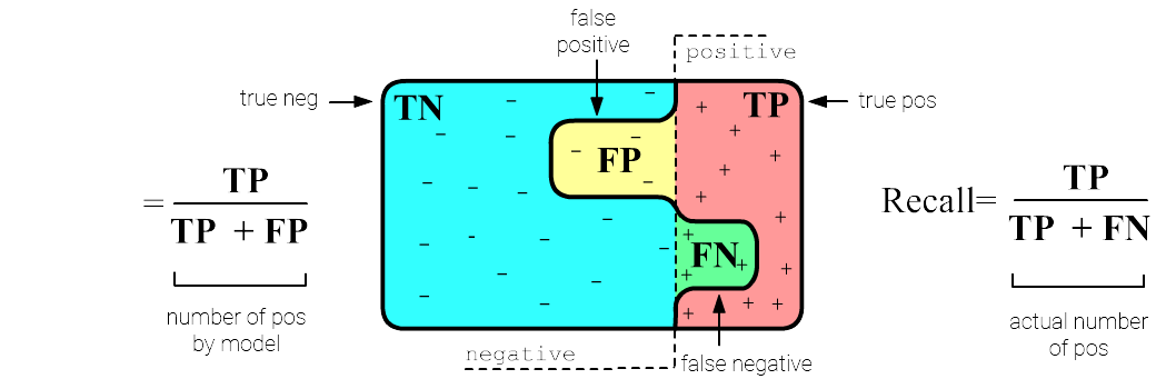
Using these definitions, we introduce two measures of model performance, with formulas shown in the image. Precision is the proportion of correct positive class predictions to the total number of positive class predictions made by the model. Recall is the similar proportion, but relative to the true number of positive examples in the data. These two measures are less sensitive to class frequency imbalance than accuracy (TN+TP)/N, where N = TN+TP + FN+FP - is the total number of examples.
Below, in a training set of 100 objects, there are 92 examples of the first class (negative) and 8 of the second (positive). The model performs very poorly in recognizing the positive class (1 correct and 7 incorrect), although the accuracy is quite high. The problem is reflected in the precision and recall:
$$ \begin{array}{|c|c|} \mathbf{N} & \mathbf{P}\\ \hline \hline \mathbf{TN} & \mathbf{FN} \\ \hline \mathbf{FP} & \mathbf{TP} \\ \hline \end{array} ~=~ \begin{array}{|r|r|} \mathbf{N} & \mathbf{P}\\ \hline 90 & ~7 \\ \hline 2 & 1 \\ \hline \end{array}~~~~~~~~~~~~ \text{Accuracy} = 0.910,~~~~~~~\text{Precision} = 0.333,~~~~~~~~~\text{Recal} = 0.125 $$Sometimes a single number is needed to measure accuracy. In this case, geometric averaging can be performed, called the F1-score:
$$ F_1 = \frac{2}{\displaystyle\frac{1}{\text{Precision}} + \frac{1}{\text{Recall}}} = \frac{\mathbf{TP}}{\mathbf{TP}+ (\mathbf{FP}+\mathbf{FN})/2} $$Different errors may have different costs depending on the task. For example, missing a sick person FN is more dangerous than a misdiagnosis FP for a healthy person. Therefore, for instance, Precision can be calculated for both positive and negative classes and summed with weights proportional to the cost of the error.
Multiple classification
Let's now consider the classification problem with the number of classes $C > 2$. In this case, the number of outputs of the model should equal the number of classes. Let the values of each $c$-th output still lie in the range [0...1] and be interpreted as the degree of confidence that an object belongs to the $c$-th class.
Classes can overlap or not overlap. In the first case, an object with features $\mathbf{x}$ can belong to multiple classes. For example, for $C=3$, the model output $\hat{\mathbf{y}}=\{0,1,1\}$ can be valid (belonging to the second and third classes, but not the first). For non-overlapping classes, any object always belongs to only one class. In this case, there are also two possibilities: strict and fuzzy classification. With strict classification, $\hat{\mathbf{y}}$ contains one unit at the $c$-th output, and zeros at the other outputs (the object definitely belongs to class $c$). With fuzzy classification, an object belongs to a single class but with a certain probability. In this case, all outputs $\hat{\mathbf{y}}$ can be non-zero, but their sum must equal one.
Classification with a large number of features can be reduced to binary classification. To do this, one needs to take $C$ models, each distinguishing "its" class from all other classes (which it does not differentiate). During testing, the most "confident" model is chosen, and it is considered that the object belongs to its class.
For non-overlapping classes, it is always possible to normalize the values of the model outputs so that their sum (for a given input) equals one. Then the output is a probability distribution over the classes.☝ If the model outputs are interpreted as probabilities, their values must lie in the interval $[0...1]$, and the sum must equal one. This can be achieved by applying the softmax function at the model's output: $$ p_i = \text{sm}(\mathbf{y}) = \frac{e^{y_i}}{\sum_k e^{y_k}},~~~~~~~~~~~~~~~~~~~~~p_i > 0,~~~~~~\sum_k p_k = 1. $$ Note that the softmax $\mathbf{p}=\text{sm}(\mathbf{y})$ is an ambiguous function. If the same number is added to each component of the vector $\mathbf{y}$, the result of the function does not change: $\text{sm}(\mathbf{y}+a) = \text{sm}(\mathbf{y})$.
y = [1, 3, 5, -3]            # model output values
p = np.exp(y)
p /= p.sum()                 # [0.016 0.117 0.867 0.   ]
Cross-entropy loss
 Let the classes be non-overlapping and it is known that the $i$-th example in the training set belongs to the class $c=c(i)$.
The model outputs are considered as class probabilities (their sum equals one).
In strict classification, the model performs better, the higher these probabilities are on average.
Therefore, as a loss function (which needs to be minimized),
we can take the negative average logarithm of the probability at the output $y_{i,с(i)}$:
$$
L = -\frac{1}{N}\sum^{N-1}_{i=0} ~ \ln y_{i,c(i)}.
$$
This error is called cross-entropy (CE).
The same formula can be applied in binary classification by having the model produce two outputs.
Let the classes be non-overlapping and it is known that the $i$-th example in the training set belongs to the class $c=c(i)$.
The model outputs are considered as class probabilities (their sum equals one).
In strict classification, the model performs better, the higher these probabilities are on average.
Therefore, as a loss function (which needs to be minimized),
we can take the negative average logarithm of the probability at the output $y_{i,с(i)}$:
$$
L = -\frac{1}{N}\sum^{N-1}_{i=0} ~ \ln y_{i,c(i)}.
$$
This error is called cross-entropy (CE).
The same formula can be applied in binary classification by having the model produce two outputs.
For $C$ classes, if the model randomly and uniformly ($y_\alpha\sim 1/C$) outputs an arbitrary class, then $L=\log C$ or $\exp(L)$ equals the number of classes. If the model works flawlessly, then $L=0$.
In the case of fuzzy classification with non-overlapping classes, one can specify the probability distribution $\hat{y}_{i\alpha}$ that the $i$-th example belongs to class $\alpha$. Then the loss function will be: $$ L = -\frac{1}{N}\sum^{N-1}_{i=0}~\sum^{C-1}_{\alpha=0} ~~\hat{y}_{i\alpha}\, \ln y_{i\alpha}. $$ Such cross-entropy between the two probability distributions $\hat{\mathbf{y}}_{\alpha}$ and $\mathbf{y}_{\alpha}$ reaches its minimum when these probabilities match. In the special case where for the $i$-th example $\hat{y}_{i\alpha}=\{0,...,0,1,0,...0\}$, where $1$ is at the position $c(i)$ if the example belongs to the class numbered $c(i)$, we return to the previous case.
For problems with overlapping classes, MSE is usually used because in this case the sum of the outputs is not equal to one. Therefore, maximizing only the probabilities of the "correct classes" does not guarantee the minimization of outputs for the "incorrect classes" (in MSE, unlike in CE, all classes are present).
Accuracy criteria in general case
When there are more than two classes, accuracy—defined as the ratio of correct classifications to the total number of examples—can still be used. However, this will be a rather coarse metric. A more detailed measure of quality is the confusion matrix:
The diagonal elements $N_{\alpha\alpha}$ - represent the number of correct predictions made by the model. Below is an example of $N_{\alpha\beta}$ for three classes. The actual number of objects in each class is 11, 14, 12. The model predicts the first class the best (first column - only one error), and the third class the worst (last column): $$ N_{\alpha\beta} ~=~ \overbrace{ \begin{array}{|c|c|c|} \hline 10 & 0 & 0 \\ \hline 1 & 11 & 4 \\ \hline 0 & 3 & 8 \\ \hline \end{array} }^{\displaystyle\text{actual}} \left. \phantom{ \begin{array}{c} \\ \\ \\ \end{array} } \right\}\text{predicted} $$
The sum of the columns equals the number of examples for a given class $N_\alpha$ (the rows represent the number of predictions made by the model): $$ N_\beta = \sum_{\alpha} N_{\alpha\beta} ~-~\text{number of examples of class $\beta$},~~~~~~~~~~~~~~N = \sum_{\alpha,\beta} N_{\alpha\beta} ~-~\text{total number of examples}. $$ The degree of "uniformity" of the frequencies $n_\alpha=N_\alpha/N$ of different class examples is characterized by the relative entropy $H$, which lies in the range [0...1]. The closer it is to one, the more balanced the examples are across $C$ classes: $$ H = -\sum_{\alpha} n_\alpha\,\log n_\alpha/\log C $$
By analogy with binary classification, metrics for precision and recall (also known as accuracy) can be introduced for each class $\alpha$: $$ P_\alpha = \frac{N_{\alpha\alpha}}{\sum_\beta N_{\alpha\beta}},~~~~~~~~~~~R_\alpha=\frac{N_{\alpha\alpha}}{N_\alpha} $$ and their average values across all classes: $$ \text{Precision} = \frac{1}{C}\sum^{C-1}_{\alpha=0} P_\alpha,~~~~~~~~~~~~~ \text{Recall} = \frac{1}{C}\sum^{C-1}_{\alpha=0} R_\alpha,~~~~~~~~~~~~ \text{Accuracy} = \frac{\sum_\alpha N_{\alpha\alpha}}{N} $$ Here is an example of calculating various metrics using Numpy:
cm = np.array([[100,  5,  0],                 # confusion matrix
              [  9,  50,  5],
              [  0,   0,  1]])

N = cm.sum()                                  # 170                 total number of examples
n = cm.sum(axis=0)/N                          # [0.641 0.324 0.035] class frequencies
H = -(n*np.log(n)).sum()/np.log(cm.shape[0])  # 0.699               entropy/log(C)

A = np.trace(cm)/N                            # 0.888  accuracy
P = (np.diag(cm)/cm.sum(axis=1)).mean()       # 0.911  precision
R = (np.diag(cm)/cm.sum(axis=0)).mean()       # 0.664  recall
There can be a situation where one class is predicted very poorly: $R_{\alpha}\sim 0$, which gets lost among the correct predictions of other classes. In this case, the relative entropy of the normalized recalls across all classes can be computed, which characterizes the "uniformity" of these recalls (accuracy of each class): $$ \text{HR} = -\sum_\alpha r_\alpha \log\,r_\alpha/\log C,~~~~~~~~~~~~~~~~~~~r_\alpha=\frac{ R_\alpha }{\sum_\beta R_\beta}. $$
For the example above:r = np.diag(cm)/cm.sum(axis=0) r = r/r.sum() HR = -(r*np.log(r)).sum()/np.log(cm.shape[0]) # 0.773
In any case, the most detailed information about the model's performance is found in the confusion matrix.
K-nearest neighbors method
 Not all models are differentiable functions of their parameters.
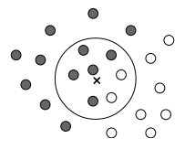
For example, consider the K-nearest neighbors method,
where instead of learning, the entire training set is memorized
(it acts as the "parameters" of the model).
When classifying a given object $\mathbf{x}$
the method examines its immediate neighborhood in the training set and makes a conclusion about
the class of the example based on this neighborhood,
such as selecting the class of the nearest neighbor.
Clearly, the quality of the method significantly depends on the correct choice
of the distance function $d(\mathbf{x},\mathbf{x}')$ between two points in the feature space.
Not all models are differentiable functions of their parameters.
For example, consider the K-nearest neighbors method,
where instead of learning, the entire training set is memorized
(it acts as the "parameters" of the model).
When classifying a given object $\mathbf{x}$
the method examines its immediate neighborhood in the training set and makes a conclusion about
the class of the example based on this neighborhood,
such as selecting the class of the nearest neighbor.
Clearly, the quality of the method significantly depends on the correct choice
of the distance function $d(\mathbf{x},\mathbf{x}')$ between two points in the feature space.
In the presence of noise, it is better to consider not just one, but K nearest neighbors $d(\mathbf{x},\mathbf{x}_1)\le d(\mathbf{x},\mathbf{x}_2)\le...\le d(\mathbf{x},\mathbf{x}_K)$ and use the class that occurs most frequently (voting). Another variation of the method consists of using neighbors within a sphere of radius R. The number K or the radius R are hyperparameters of the method.
Hyperparameter tuning can be performed using the LOO (leave-one-out) method. In this approach, the neighbors method is applied sequentially to each object in the training set (the current object is naturally not considered among its own neighbors). The hyperparameter value that results in the highest class recognition accuracy is selected.
Training, testing and validation
As previously mentioned, model parameter selection must be conducted on training data (by minimizing the loss function) and the accuracy should be checked on test data. Generally, data is divided into three sets: train, validation and test sets:

The validation set is used to check the model for overfitting. If the error decreases and accuracy increases on the training data, but the opposite happens on the validation data, it is necessary to reduce the number of parameters or change the model. The test data does not participate in these iterations of model selection and training. They are used to assess the quality of the final model.
Validation data can also be used for hyperparameter tuning. There are several ways to split data into training and validation sets. In a simple split the original data is randomly shuffled and a certain portion (e.g., 25%) is designated for validation.
A more general method is cross-validation. The training data is divided into q roughly equal blocks. First, the first block is chosen as the validation set and the rest are used for training. Then, the second block is used for validation, and so on.
This procedure can be repeated t times, with the data randomly shuffled each time, which is known as the (t x q) - fold cross-validation method. The model accuracy is averaged across all blocks and repetitions. The leave-one-out method is a special case where t=1 and q=N-1, where N is the number of examples.
Feature engineering
If the features characterizing an object are chosen correctly, the machine learning task becomes trivial. Let's consider a classic example. In the two-dimensional feature space below, we need to classify two classes (squares and circles). On the left image, the features are Cartesian coordinates $\{x_0,x_1\}$, and the separating surface is a circle: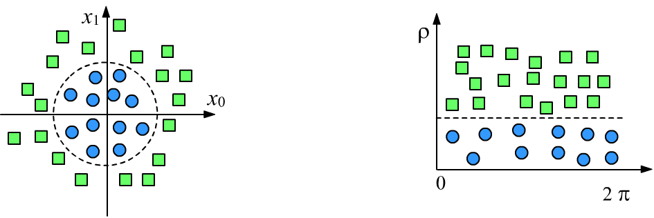
In the past, significant efforts were directed towards finding various ways to construct good features for objects. Nowadays, it is believed that this is not necessarily required, as deep neural networks "themselves" form the most effective object descriptions in their final layer during training.
Despite the obvious successes of this approach,
preparing good features for model training is still beneficial.
In particular, it is usually worth at least normalizing
the input data.
For this, the mean $\bar{x}_\alpha$ and variance
$\sigma^2_\alpha$ of each feature are computed across all examples, and new features are derived:
$$
x_{i\alpha} \mapsto \frac{x_{i\alpha}- \bar{x}_\alpha}{\sigma_\alpha},~~~~~~~~~~~~~~~~\bar{x}_\alpha=\frac{1}{N}\sum^{N-1}_{i=0} x_{i\alpha},~~~~~~~~
\sigma^2_\alpha =\frac{1}{N-1}\sum^{N-1}_{i=0}(x_{i\alpha}-\bar{x}_\alpha)^2.
$$
Thus, normalized features will have the same scale, which can simplify training.
In conclusion, let us recall an old parable:
Once upon a time, Jed and Ned wanted to distinguish their horses. Jed made a scratch on the ear of his horse. But Ned's horse scratched the same ear on a thorn. Then Ned attached a blue ribbon to his horse's tail, but Jed's horse ate it. The farmers thought for a long time and chose a feature that was not so easy to alter. They carefully measured the height of the horses, and it turned out that Jed's black mare was one centimeter taller than Ned's white stallion.
