ML: Word Embeddings
Introduction
Let's list all values of a qualitative feature in the $\mathcal{V}$ (vocabulary)
of size V_DIM = V.
For example, for 7 colors
{red, green, blue, yellow, cyan, magenta, gray} the vocabulary size is V = 7.
In order for a neural network to work with such a feature, it must be vectorized.
This means that each feature value is mapped to a unique vector
with E_DIM = E components.
Thus, a qualitative feature is effectively embedded into a real-valued vector space.
Each feature value corresponds to a point in an E-dimensional space.
The coordinates of this point (real numbers) can be fed into a neural network or any other machine learning model.
When the number of feature values is small, one-hot encoding is suitable. In this case, the vector dimensionality equals the vocabulary size (E = V), and the vector of the i-th word consists of zeros except for a single one at position i. One-hot encoding can be interpreted as a V-dimensional space where each axis represents the presence (1) or absence (0) of a particular value. All word vectors in the vocabulary are pairwise orthogonal:
Vocabulary      One-hot                Embedding
------------------------------------------------------
1. red        [1, 0, 0, 0, 0, 0, 0]    [1.0, 0.0, 0.0]
2. green      [0, 1, 0, 0, 0, 0, 0]    [0.0, 1.0, 0.0]
3. blue       [0, 0, 1, 0, 0, 0, 0]    [0.0, 0.0, 1.0]
4. yellow     [0, 0, 0, 1, 0, 0, 0]    [1.0, 1.0, 0.0]
5. cyan       [0, 0, 0, 0, 1, 0, 0]    [1.0, 0.0, 1.0]
6. magenta    [0, 0, 0, 0, 0, 1, 0]    [0.0, 1.0, 1.0]
7. gray       [0, 0, 0, 0, 0, 0, 1]    [0.2, 0.2, 0.2]
One-hot encoding is sometimes also used for natural language words, even though the vocabulary can be very large.
Any document can be represented as the sum (or logical OR) of the one-hot vectors of its words.
Such a document vector is called a bag of words (BoW),
because it reflects only the number or presence (with OR) of words in the document, but not their order.
This simple vectorization can be used, for example, for document classification or search.
One-hot encoding has two major drawbacks: 1) for large vocabularies, vector representations become very high-dimensional, increasing the number of model parameters; 2) one-hot vectors do not reflect semantic similarity between different words (if such similarity exists).
To overcome these limitations, vectors of relatively small dimensionality with real-valued components are used. Most components are non-zero, making this a distributed representation encoding. This approach is called Embedding or Word2Vec. The vector components are usually learned during training. It is assumed that vectors in the E-dimensional space will form clusters according to semantic similarity, which simplifies the training of subsequent model layers. However, embeddings can also be predefined (as in the example above, these are {R,G,B} color components).
For experiments with natural language word vectorization, we need a text corpus. We will use short stories from the ROC Stories dataset. A detailed description can be found in NLP_ROCStories.html. The examples use the PyTorch library and are provided in the notebook NN_Embedding_Learn.ipynb. The notebook requires texts from the file 100KStories.csv. A lightly cleaned version of the stories can be downloaded from our website.
Context vectors
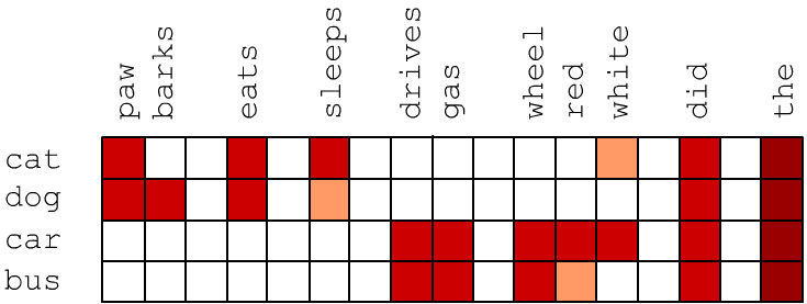
For each word $w_i$ in the vocabulary $\mathcal{V}$, we want to associate a vector $\mathbf{u}_i=\{u_{i0},...,u_{i,\text{E}-1}\}$ such that semantically similar words have similar vectors. As a result, for example, the words dog, cat, rabbit should be located close to each other in the vector space (forming a cluster), and at the same time be far away from the cluster of words car, bus, train.
Semantic similarity between two words implies that in texts they occur in similar contexts, i.e. on average they are surrounded by the same words. Let's first consider vectors of dimensionality E_DIM equal to the number of words V_DIM in the vocabulary (E=V). Let the j-th component of the vector of the i-th word be proportional to the frequency $u_{ij} = P(w_i,w_j)$ of joint occurrence of words $w_i$ and $w_j$ in the same sentence. Semantically close words may not necessarily appear in the same sentence, but they share similar contexts and therefore have similar vectors. Below, high values of $P(w_i,w_j)$ are schematically highlighted in red. It is clear that the vectors of cat and dog are similar and differ from the vectors of car and bus:
Joint word occurrence frequencies in natural language are "noisy" due to very frequent words such as the article 'the' (Zipf’s law). To reduce this effect, instead of raw frequency we use the pPMI (positive pointwise mutual information) metric: $$ \mathrm{pPMI} = \max(0,\,\mathrm{PMI}),~~~~~~~~~~~~\mathrm{PMI} = \log \frac{P(w_1, w_2)}{P(w_1)P(w_2)} ~\equiv~ \log \frac{P(w_1\,|\,w_2)}{P(w_1)}. $$ If words $w_1$ and $w_2$ are "independent", then the conditional probability $P(w_1\,|\,w_2)=P(w_1)$, and and the joint probability $P(w_1, w_2) \,=\, P(w_1)P(w_2)$. In this case $\mathrm{PMI}=0$. The $\max$ function in the definition of pPMI clips zero joint probabilities and possible negative logarithm values when $P(w_1\,|\,w_2) < P(w_1)$.
Below is one way to compute the joint probability of two words appearing in the same sentence using the numpy library. Loading the list of docs (ROC Stories) and building the vocabulary wordID are described in ROC Stories.
import numpy as np

p12 = np.zeros((V_DIM, V_DIM))                   # joint probabilities
p1  = np.zeros((V_DIM,))                         # word frequencies

for d in docs:                                   # iterate over documents
    for s in d:                                  # iterate over sentences
        ws = set(s.split())                      # set of words in sentence
        for w1 in ws:
            if w1 in wordID:                     # word exists in vocabulary
                p1[ wordID[w1]["id"] ] += 1
                for w2 in ws:
                    if w2 in wordID:
                        p12[ wordID[w1]["id"], wordID[w2]["id"] ] += 1

p12 /= p12.sum()                                 # normalize
p1  /= p1.sum()
Now we can compute word vectors using the pPMI formula:
vecs = p12 / ( p1.reshape((V_DIM,1)) @ p1.reshape((1, V_DIM)) )

vecs[vecs <= 0] = 1                              # zeros or negatives under log
vecs = np.log(vecs)
vecs[vecs <= 0] = 0                              # max in pPMI
Computing vector components for the 100k ROCStories corpus in Python takes about one minute (on CPU Intel i7-7500U 2.7GHz, 16Gb). Below are examples of several components of four vectors (zeros omitted):
         paws       vet     wheel      driver   motion     white      very      we        can
     bark     collar    claw       gas      stops      red       the       after    not        to
    ------------------------------------------------------------------------------------------------
cat  1.1  4.0  2.6  2.9  2.5                                1.6  0.4  0.3       0.1
dog  3.7  2.9  3.3  3.0                      0.2            1.1  0.4       0.1            0.1

car                           1.5  2.2  2.0  1.5       1.3       0.3            0.1            0.1
bus                                     3.8  2.7  2.6            0.8       0.5  0.4            0.3

say  2.7                                0.5                 0.5                 0.4  1.1  1.3  0.8
ask                                1.7       2.1                                     0.2  1.1  1.1
get                 0.9       0.8  1.0       0.9  1.2                           0.3  0.7  0.7  1.0
Note the small pPMI values associated with high-frequency words values associated with high-frequency words. Obviously, these words have no direct semantic relationship with cat, dog, cat, bus.
Dimensionality reduction
Although the components of word vectors now reflect word similarity, their dimensionality is still as large as with one-hot encoding. To reduce the dimensionality of the embedding, we use principal component analysis (PCA):
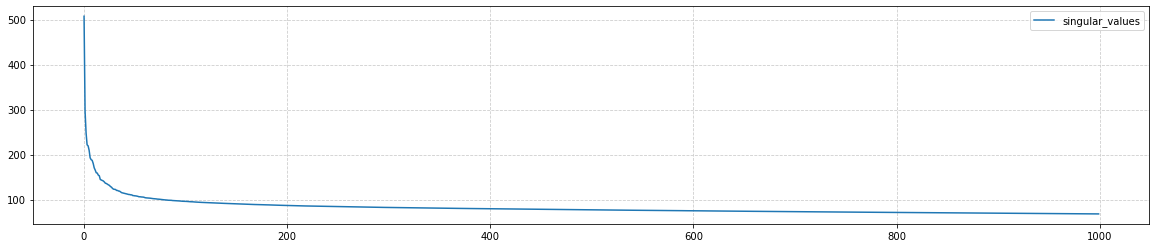
from   sklearn.decomposition import PCA

pca = PCA()
res = pca.fit_transform(vecs)
Computing principal components for a matrix of size (10000, 10000) takes about 7 minutes. The first 50 eigenvalues of the covariance matrix (pca.singular_values_) decrease rapidly, and then the decay toward zero (at i=V) becomes almost linear:
We further restrict the vector space dimensionality to E_DIM = E = 100:
vecs = res[:, : E_DIM]                                           # first 100 columns
vecs = (vec-vec.mean(axis=0))/(res.std(axis=0) * np.sqrt(E_DIM) )# normalize variance
Final normalization of the components (subtracting the mean and dividing by the standard deviation) moves the "center of the point cloud" to the origin, which improves the performance of the cosine similarity measure (see below). Dividing by the square root of the embedding dimensionality E_DIM scales vector lengths to be approximately unit on average.
Similarity measures
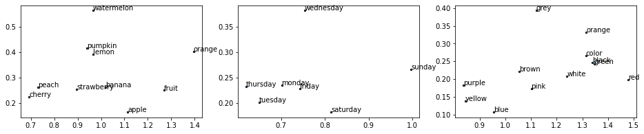
Similarity measures between two vectors $\mathbf{u}$, $\mathbf{v}$ in a multidimensional space can be defined in different ways: $$ \begin{array}{llclcl} \text{Euclidean distance:} & \text{dist}_1(\mathbf{u},\mathbf{v}) &=& \sqrt{(\mathbf{u}-\mathbf{v})^2}\\[2mm] \text{Cosine distance:} & \text{dist}_2(\mathbf{u},\mathbf{v}) &=& 1-\cos(\mathbf{u},\mathbf{v})&=& 1-\displaystyle \frac{\mathbf{u}\mathbf{v}}{|\mathbf{u}|\cdot|\mathbf{v}|} \end{array} $$ After dimensionality reduction, cosine distance is used more often. Using cosine distance, we find the nearest neighbors for several words (see module my_embedding.py):
- cat: kitten (0.17), dog (0.18), puppy (0.25), kittens (0.32), stray (0.33), pet (0.33), poodle (0.34), pup (0.36), chihuahua (0.36), shelter (0.37), meowed (0.37), cats (0.38), kitty (0.39)
- car: truck (0.23), vehicle (0.28), driving (0.30), cars (0.30), driver (0.32), road (0.33), intersection (0.33), interstate (0.33), tire (0.34), brakes (0.34), semi (0.34), towed (0.34), sped (0.35), highway (0.36), rear-ended (0.38), ford (0.39), van (0.39), swerved (0.39), wrecked (0.40), oncoming (0.40), drivers (0.41), parked (0.41)
- apple: orchard (0.30), peach (0.31), apples (0.32), blueberry (0.34), pie (0.34), fruit (0.37), cherry (0.37), banana (0.42), oranges (0.43), bakes (0.46), peaches (0.46), bake (0.48), dessert (0.48), ripe (0.48), fresh (0.49), smoothie (0.49), picking (0.49), grapes (0.49), pumpkin (0.49), pies (0.49), muffins (0.51), bananas (0.51), lemon (0.52), cherries (0.53)
- gin: vodka (0.27), martini (0.32), drink (0.32), drank (0.34), drinking (0.38), drinks (0.40), wine (0.40), iced (0.41), sipping (0.41), champagne (0.43), beer (0.43), bartender (0.45), whiskey (0.46), beers (0.47), alcoholic (0.48), espresso (0.49), decaf (0.49), sipped (0.49), soda (0.50), beverage (0.50), tea (0.50), sip (0.50), glass (0.51), coffee (0.51)
- monday: tuesday (0.39), saturday (0.47), early (0.48), wednesday (0.48), friday (0.50), overslept (0.50), thursday (0.51), morning (0.52), late (0.52), noon (0.54), sunday (0.55), meeting (0.55), today (0.55), pm (0.57), scheduled (0.57), :30 (0.58), appointment (0.59), 11 (0.60), lecture (0.61), postponed (0.62), woke (0.62), 8 (0.62), arrive (0.62), april (0.63)
- red: blue (0.23), yellow (0.29), bright (0.31), stripes (0.34), white (0.37), pale (0.38), purple (0.42), brown (0.42), pink (0.43), flashing (0.43), green (0.43), colored (0.44), resulting (0.47), black (0.47), puffy (0.48), orange (0.50), dyed (0.51), streaks (0.51), color (0.52), dye (0.53), eyes (0.53), stains (0.54), ink (0.54), stained (0.55)
- small: large (0.39), a (0.46), big (0.46), suburban (0.52), huge (0.54), tiny (0.55), near (0.58), breeder (0.59), stone (0.59), sized (0.60), cardboard (0.61), own (0.61), inheritance (0.62), corgi (0.64), larger (0.64), little (0.64), lived (0.65), isolated (0.66)
- say: [seem (0.43), tell (0.43), know (0.46), anything (0.46), understand (0.48), what (0.48), happen (0.49), exist (0.49), matter (0.50), psychic (0.50), saying (0.50), don't (0.51), anybody (0.51), hello (0.51), why (0.52)', won't (0.52), god (0.52), cruel (0.54), hi (0.54), respond (0.54), says (0.55), ? (0.55), sorry (0.56), yes (0.56)
For comparison, cosine and Euclidean distances between these words:
                        dist_cos                                              dist_len
       cat    car  apple gin  monday red   small say        cat    car  apple gin  monday red   small say
cat          0.94  1.01  0.90  1.07  1.02  0.84  1.01             2.62  2.62  1.98  2.27  3.06  2.46  2.32
car    0.94        0.97  1.07  1.06  0.87  1.02  1.02       2.62        2.57  2.10  2.26  2.83  2.73  2.33
apple  1.01  0.97        0.99  0.94  0.84  0.94  1.03       2.62  2.57        1.90  2.02  2.70  2.51  2.22
gin    0.90  1.07  0.99        1.16  0.90  1.01  1.09       1.98  2.10  1.90        1.40  2.38  2.03  1.53
monday 1.07  1.06  0.94  1.16        0.89  1.09  1.15       2.27  2.26  2.02  1.40        2.48  2.27  1.81
red    1.02  0.87  0.84  0.90  0.89        0.98  1.05       3.06  2.83  2.70  2.38  2.48        2.98  2.73
small  0.84  1.02  0.94  1.01  1.09  0.98        1.04       2.46  2.73  2.51  2.03  2.27  2.98        2.33
say    1.01  1.02  1.03  1.09  1.15  1.05  1.04             2.32  2.33  2.22  1.53  1.81  2.73  2.33
Note that the cosine distance between words from different clusters is on the order of one,
which indicates near-orthogonality of these vectors.
Compared to neural-network-based approaches, vectorization using PCA is a relatively fast method and, for moderately sized vocabularies, can serve as a very good first approximation.
Properties of vector space
Let's construct histograms of vector length distributions separately for frequent words (the first 1000), rare words, and all words together. Frequent words have longer vectors, which is typical for all embedding methods: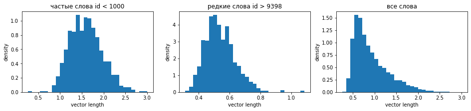
Semantic directions
Let's compute the difference vector between the vectors of two words $\mathbf{u}_1-\mathbf{u}_2$. We report its length len and the matrix of cosine distances between such vectors (if they are smaller than 1, the angle between the vectors is less than 90°):
        sex                   pm          len      1      2      3      4      5      6      7
1. [he          she    ]   23352 - 19702| 0.63|        0.56   0.60   0.44   0.68   0.71   0.84
2. [man         woman  ]    1020 -   311| 1.35| 0.56          0.57   0.74   0.84   0.91   0.75
3. [boy         girl   ]     378 -   551| 1.18| 0.60   0.57          0.78   0.85   0.77   0.76
4. [father      mother ]     319 -   744| 1.43| 0.44   0.74   0.78          0.64   1.06   1.13
5. [uncle       aunt   ]      68 -    76| 1.34| 0.68   0.84   0.85   0.64          0.95   1.10
6. [nephew      niece  ]      38 -    65| 1.18| 0.71   0.91   0.77   1.06   0.95          0.87
7. [king        queen  ]      29 -    17| 1.00| 0.84   0.75   0.76   1.13   1.10   0.87
The age axis is noticeably weaker:
         age               pm             len      1      2      3      4      5
1. [old          young ]     778 -   175| 2.23|        0.99   0.93   1.05   1.09
2. [man         boy    ]    1020 -   378| 1.81| 0.99          0.32   0.94   0.92
3. [woman       girl   ]     311 -   551| 1.58| 0.93   0.32          0.97   0.94
4. [grandpa     dad    ]      56 -   568| 1.54| 1.05   0.94   0.97          0.66
5. [grandmother mother ]     120 -   744| 1.45| 1.09   0.92   0.94   0.66
A bit of Math $^*$
Recall that the PCA method in $n$-dimensional space seeks
the "closest" $m$-dimensional plane to the training points,
for which the mean squared deviation of the point distances is minimal.
The coordinates of $N$ points in $n$-dimensional space are given by the matrix $\mathbf{X}$ of shape $(N,n)$.
Assume the mean of each coordinate over all points has been subtracted.
Then the covariance matrix is $\mathbf{C} = \mathbf{X}^\top\mathbf{X}/(N-1)$.
The solution of the PCA-problem reduces to finding the eigenvalues $\lambda_1 \ge ... \ge \lambda_n$ of the covariance matrix $\lambda_\alpha$: $\mathbf{C}\,\mathbf{v}^{(\alpha)}=\lambda_\alpha\,\mathbf{v}^{(\alpha)}.$ Let $\mathbf{L}=\text{diag}(\lambda_1,...\lambda_n)$ be a diagonal matrix. Then $\mathbf{C}=\mathbf{V}\mathbf{L}\mathbf{V}^\top$, where each column of matrix $\mathbf{V}_{i\alpha}=v^{(\alpha)}_i$ contains components of the eigenvectors $\mathbf{v}^{(\alpha)}.$ The first $m$ columns of $\mathbf{X}\mathbf{V}$ of shape $(N,n)$ are the coordinates of the projections of points $\mathbf{X}$ onto the $m$-dimensional plane.
When computing $\mathbf{C}$, multiplying large matrices $\mathbf{X}$ of shape $(N,n)$ can lead to numerical precision loss. Therefore, it is sometimes more efficient to use SVD (singular value decomposition):

where $\mathbf{S}$ is a diagonal matrix $(N,n)$ with singular values $s_i$ with singular values, and $\mathbf{U}, \mathbf{V}$ are orthogonal matrices (columns of $\mathbf{U}$ are eigenvectors of $\mathbf{X}\mathbf{X}^\top$, and columns of $\mathbf{V}$ are eigenvectors of $\mathbf{X}^\top\mathbf{X}$). Thus,
$$ \mathbf{C} = \frac{\mathbf{X}\mathbf{X}^\top}{N-1} = \frac{\mathbf{V}\mathbf{S}\mathbf{U}^\top\,\mathbf{U}\mathbf{S}\mathbf{V}^\top} {N-1} =\mathbf{V}\frac{\mathbf{S}^2}{N-1}\mathbf{V}^\top. $$Hence, the eigenvalues of the covariance matrix are $\lambda_i=s^2_i/(N-1)$, and the principal components are given by $\mathbf{X}\mathbf{V}=\mathbf{U}\mathbf{S}\mathbf{V}^\top\mathbf{V}=\mathbf{U}\,\mathbf{S}$. In numpy, PCA using SVD is performed as follows:
U, S, V = np.linalg.svd(X - X.mean(axis=0))
vecs = U[:, : m] @ np.diag(S[ : m])

Global Vectors (GloVe)
For very large vocabularies, dimensionality reduction using PCA or SVD can be difficult. In such cases, neural networks are often used, which directly operate in low-dimensional vector spaces (see the next document). In the paper Pennington J. et.al. (2014) an intermediate approach called "Global Vectors for Word Representation" (GloVe) was proposed.
In this approach, first the logarithms of co-occurrence probabilities $P_{ij}$ of words $w_i$ and $w_j$ within a sliding window of 10 words are computed. The trainable parameters are the E-dimensional word vectors $\mathbf{u}_i$ and bias terms $b_i$. During training, (selection of $\mathbf{u}_i$ and $b_i$) the following loss function is minimized:
$$ \text{Loss} = \sum_{ij} f(N_{ij})\,\bigr(\mathbf{u}_i\mathbf{u}'_j + b_i + b'_j - \log P_{ij}\bigr)^2 = \min_{\mathbf{u}_i,\mathbf{u}'_j\,b_i,b'_j} $$ The weights $f(N_{ij})$ are proportional to the number of occurrences $N_{ij}$ of the pair in the window. These weights are clipped for very frequent words. The authors chose the following function with $x_\text{max}=100$ independent (?) of text length.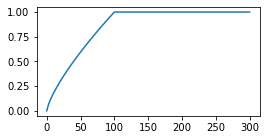 $$
f(x) =
\left\{
\begin{array}{ll}
(x/x_{\text{max}})^{3/4} & \text{if}~ x < x_{\text{max}}\\
1 & \text{otherwise}
\end{array}
\right.
$$
$$
f(x) =
\left\{
\begin{array}{ll}
(x/x_{\text{max}})^{3/4} & \text{if}~ x < x_{\text{max}}\\
1 & \text{otherwise}
\end{array}
\right.
$$
Different vectors $\mathbf{u}$ and $\mathbf{u}'$ are used in the dot product $\mathbf{u}_i\mathbf{u}'_j$, and the final embedding is $\mathbf{u}+\mathbf{u}'$. According to the authors, this helps prevent overfitting (even though $P_{ij}=P_{ji}$, the initial random values of $\mathbf{u}$ and $\mathbf{u}'$ are different). The bias parameters $b_i$, $b'_j$ can be interpreted as trainable probabilities in the denominator ofPMI, i.e., minimizing the loss approximates $\mathbf{u}_i\mathbf{u}'_j = \log P_{ij}/P_i P_j$.
The vectors were trained on large text corpora:
We trained our model on five corpora of varying sizes: a 2010 Wikipedia dump with 1 billion tokens; a 2014 Wikipedia dump with 1.6 billion tokens; Gigaword 5 which has 4.3 billion tokens; the combination Gigaword5 + Wikipedia2014, which has 6 billion tokens; and on 42 billion tokens of web data, from Common Crawl
Publicly available vector sets have dimensions from 50 to 300 and a vocabulary of 400k. Before constructing the vocabulary, the authors "tokenize and lowercase each corpus with the Stanford tokenizer". It is a good idea to also use the Stanford tokenizer with GloVe, since it handles contractions: can't → [ca, n't]; she's → [she, 's], etc.Analysis of the GloVe vector space can be found in this document.
Embedding problems
Embedding technology is one of the most remarkable inventions of the last decade. However, it also comes with several issues.
✑ To obtain reliable contextual vectors for rare words, a very large text corpus is required. However, in a large corpus, there may be a bias in the semantic meanings of words compared to their typical everyday meanings. For example, when vectorizing GloVe for the word apple, the nearest neighbors might be: microsoft(.26), ibm (.32), intel(.32), software(.32), dell (.33). At the same time, a significantly smaller corpus like ROC Stories produces more "everyday" neighbors for apple.
✑ Simple embeddings do not account for semantic and syntactic ambiguity. It is usually assumed that semantic ambiguity is resolved after passing the initial word vectors through several layers of a neural network, where the context of the entire sentence is analyzed (architectures like RNN or Attention). For example, the overall context of the sentences "Remove first row of the table." and "Put an apple on the table" allows disambiguating the semantic meaning of the word table in each case.
✑ Since words in vector space are points and not extended regions, embeddings do not reflect the hierarchical nature of meanings: object - tool - hammer.
