ML: Introduction to PyTorch: 3. Neural Networks
Sequence of layers
This document discusses how to create and train neural networks using the PyTorch library, the basics of which are described here and here. A reference guide for the main types of layers, losses, and optimizers can be found here.
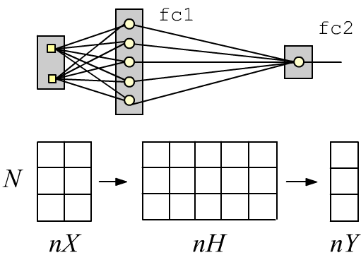
Simple neural networks with a sequential architecture can be created using the stack-style interface. For example, a two-layer fully connected network with two inputs (nX=2 features), one (nY=1) sigmoid output (2 classes), and five neurons (nH=5) in the hidden layer can be defined as follows:
import torch
import torch.nn as nn

nX, nH, nY = 2, 5, 1

model = nn.Sequential(
          nn.Linear(nX, nH),    # the first layer
          nn.Sigmoid(),         # hidden layer activation
          nn.Linear(nH, nY),    # the second, output layer
          nn.Sigmoid() )        # its activation function
The Linear layer performs a linear transformation of an input tensor with shape (N, nX), where N is the number of examples. At the output of this layer, we obtain a tensor of shape (N, nH), which is then passed through a sigmoid (producing new nH features). The second layer produces a tensor of shape (N, nY), which is also passed through a sigmoid. If its value is less than 0.5 - it belongs to the first class; if greater than 0.5 - it belongs to the second.
Functional architecture
When designing complex neural networks, it is often more convenient to define their architecture in a functional form.
To do this, a subclass of nn.Module is created.
In this subclass, the constructor and the forward method are redefined.
In the constructor, the required layers are specified and their parameters are initialized.
Note the call to the parent class constructor, to which it is necessary to pass the name of our class.
In the forward method (forward propagation), the architecture of the network is defined
(the layers are linked together into a computational graph):
class TwoLayersNet(nn.Module):
    def __init__(self, nX, nH, nY):
        super(TwoLayersNet, self).__init__()     # parent constructor with this class name

        self.fc1 = nn.Linear(nX, nH)             # create model parameters
        self.fc2 = nn.Linear(nH, nY)             # in fully connected layers

    def forward(self, x):                        # define forward pass
        x = self.fc1(x)                          # output of the first layer
        x = nn.Sigmoid()(x)                      # pass through Sigmoid
        x = self.fc2(x)                          # output of the second layer
        x = nn.Sigmoid()(x)                      # pass through Sigmoid again
        return x

model = TwoLayersNet(2, 5, 1)                    # create a network instance
The call nn.Linear(in_features, out_features) creates two instances of fully connected linear layers fc1, fc2. At the same time, random values are assigned to their weights and biases. The parenthesis operator fc1(x) inside the forward method executes the computations within the layer and outputs the resulting tensor.
Model data
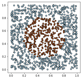 Let's create model data in PyTorch for two types of objects (two classes)
characterized by two features. Suppose on a 2D plane,
objects of the first class fill the unit square $[0...1]^2$, except for a circle in the center of the square,
where objects of the second class are located:
Let's create model data in PyTorch for two types of objects (two classes)
characterized by two features. Suppose on a 2D plane,
objects of the first class fill the unit square $[0...1]^2$, except for a circle in the center of the square,
where objects of the second class are located:
X = torch.rand (1200,2)
Y = (torch.sum((X - 0.5)**2, axis=1) < 0.1).float().view(-1,1)
Using the matplotlib library, we can visualize the generated data:
import matplotlib.pyplot as plt                              # plotting library

plt.figure (figsize=(5, 5))                                  # figure size (square)
plt.scatter(X.numpy()[:,0], X.numpy()[:,1], c=Y.numpy()[:,0],
            s=30, cmap=plt.cm.Paired, edgecolors='k')
plt.show()                                                   # display the plot
Network training
To train the network, you need to create a loss function (what should be minimized) and an optimizer (which will minimize this loss). The optimizer receives the model parameters. As the loss, we choose binary cross-entropy (BCELoss), and the optimizer will be SGD (Stochastic Gradient Descent):
model = TwoLayersNet(2, 5, 1)                            # network instance

loss      = nn.BCELoss()
optimizer = torch.optim.SGD(model.parameters(),          # model parameters
                            lr=0.5, momentum=0.8)        # optimizer settings
On each iteration, a batch array is formed from the training samples,
then forward propagation is executed
y = model(bx) and
the loss is computed (by comparing the model output y with the correct labels yb).
On the computational graph of the loss, the method loss.backward() computes
the gradients of the model parameters, which the optimizer uses in the step()
method to update the parameter values:
def fit(model, X,Y, batch_size=100, train=True):
      model.train(train)                                 # important for Dropout, BatchNorm
      sumL, sumA, numB = 0, 0, int( len(X)/batch_size )  # loss, accuracy, batches

      for i in range(0, numB*batch_size, batch_size):
        xb = X[i: i+batch_size]                          # current batch
        yb = Y[i: i+batch_size]                          # X,Y are torch tensors

        y = model(xb)                                    # forward propagation
        L = loss(y, yb)                                  # compute loss

        if train:                                        # training mode
            optimizer.zero_grad()                        # reset gradients
            L.backward()                                 # compute gradients
            optimizer.step()                             # update parameters

        sumL += L.item()                                 # total loss (item from graph)
        sumA += (y.round() == yb).float().mean()         # classification accuracy

    return sumL/numB,  sumA/numB                         # average loss and accuracy
The fit function makes a pass through all the data. This is called a training epoch. If the parameter leran=True is set, the model is trained (its parameters are updated). The value leran=False is used when evaluating the model quality without changing it. As quality metrics, the average loss over all examples and the average accuracy (the proportion of correctly predicted classes) are used. Usually, a sufficiently large number of training epochs is required:
                                                         # model evaluation mode:
print( "before:      loss: %.4f accuracy: %.4f" %  fit(model, X,Y, train=False) )

epochs = 1000                                            # number of epochs
for epoch in range(epochs):                              # an epoch - pass through all examples
    L,A = fit(model, X, Y)                               # one epoch

    if epoch % 100 == 0 or epoch == epochs-1:
        print(f'epoch: {epoch:5d} loss: {L:.4f} accuracy: {A:.4f}' )
As a result, we will obtain something like:
before:      loss: 0.6340 accuracy: 0.6950
epoch:     0 loss: 0.6327 accuracy: 0.6550
....
epoch:   999 loss: 0.0334 accuracy: 0.9908
To improve training, it is usually recommended to shuffle the data. This can be done in two ways. The first method is executed before the fit function at the beginning of each epoch:
    idx = torch.randperm( len(X) )     # Shuffled index list
    X = X[idx]
    Y = Y[idx]
In this method, new memory is allocated for all the data, which is not always optimal for large training sets.
The second method performs a random sampling only for the current batch inside the
fit function:
    idx = torch.randint(high = len(X), size = (batch_size,) )
    xb = X[idx]
    yb = Y[idx]
This method uses less memory, but during a single epoch not all samples may be used for training,
and the same samples may appear in a batch.
This method is used in the DataLoader class (the shuffle parameter), see below.
Thus, compared to Keras in TensorFloor, the training procedure must be written manually. However, in complex cases this allows you to intervene in the process at any stage. For example, you can insert your own optimizer :)
.       if train:                                        # in training mode
            L.backward()                                 # compute gradients
            with torch.no_grad():
                for p in model.parameters():
                    p.add_(p.grad, alpha=-0.7)           # p += -0.7*grad
                    p.grad.zero_()
Network structure output
The easiest way to see the network layers is to just print the model:
print(model) # textual representation of the model
It is more convenient to use the external modelsummary module. Its summary function is given an input tensor with any values (but with the correct shape) from a single example (the first dimension in shape will be -1):
from modelsummary import summary

summary(model, torch.zeros(1, 2), show_input=False)      # analogous to summary in keras
-----------------------------------------------------------------------
             Layer (type)               Output Shape         Param #
=======================================================================
                 Linear-1                    [-1, 5]              15
                 Linear-2                    [-1, 1]               6
=======================================================================
Total params: 21
Trainable params: 21
Non-trainable params: 0
If you set show_input=True, then instead of the output shape,
the input shape of each layer will be printed.
For composite models, you can run the summary function
with the parameter show_hierarchical=True.
for layer in model:
    print("***", layer)
    for param in layer.parameters():
        print(param.data.numpy())
 In general, the model parameters are derived as follows:
for param in model.parameters():
    print(param.numel(), param.size(), param.data.numpy())
tot = 0
for k, v in model.state_dict().items():
    pars = np.prod(list(v.shape)); tot += pars
    print(f'{k:20s} :{pars:7d}  shape: {tuple(v.shape)} ')
print(f"{'total':20s} :{tot:7d}")
fc1.weight           :     10  shape: (5, 2)
fc1.bias             :      5  shape: (5,)
fc2.weight           :      5  shape: (1, 5)
fc2.bias             :      1  shape: (1,)
total                :     21
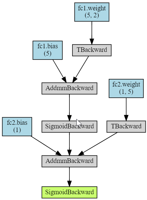
Finally, the torchviz library allows you to visualize the computational graph of the model (image on the right):
import torchviz

torchviz.make_dot(model(X),
                  params = dict(model.named_parameters()) )
The AddmmBackward node corresponds to the torch.addmm(v, m1, m2, b=1, a=1) function, which multiplies matrices and adds a vector to them: b v + a (m1 @ m2).
Saving and loading
The torch.save method saves any dictionary in binary form, including the state of the model and the optimizer:
import datetime

state = {'info':      "This is my network",      # description
         'date':      datetime.datetime.now(),   # date and time
         'model' :    model.state_dict(),        # model parameters
         'optimizer': optimizer.state_dict()}    # optimizer state

torch.save(state, 'state.pt')                    # save the file
They can then be loaded after creating the model and optimizer beforehand (their parameters can be arbitrary,
since they will be loaded from the file):
state = torch.load('state.pt')                   # load the file

m = TwoLayersNet(2, 5, 1)                        # network instance
optimizer = torch.optim.SGD(m.parameters(),lr=1) # optimizer (any parameters)

m.        load_state_dict(state['model'])        # load model parameters
optimizer.load_state_dict(state['optimizer'])    # load optimizer state

print(state['info'], state['date'])              # auxiliary information
Dataset classes
In PyTorch, it is customary to wrap training data in a class. It inherits from the Dataset class and overrides the __len__ method (the number of samples) and the __getitem__ method for retrieving a sample by index idx:
class MyDataset(torch.utils.data.Dataset):       # Inherits from Dataset

    def __init__(self, N = 10, *args, **kwargs):
        super().__init__(*args,**kwargs)

        self.x = torch.rand(N,1)                 # random data

    def __len__(self):                           # Number of samples
        return len(self.x)

    def __getitem__(self, idx):                  # get the idx-th sample
        return {'input' : self.x[idx],
                'target': 2*self.x[idx]}


data = MyDataset()

for sample in data:
    print(sample)      # {'input': tensor([0.1545]), 'target': tensor([0.3090])} ...
After creating a dataset, it can be passed to a DataLoader object,
which will provide batches, shuffle, split into training and test sets, normalize data, etc.
(see the documentation).
train_loader = torch.utils.data.DataLoader(dataset=data, batch_size=12, shuffle=False)

for batch in train_loader:                       # get batches for training
    print(batch['input'], batch['target'])
GPU computing
To perform computations on a GPU (as in the general case), it is necessary to create the corresponding devices:
gpu = torch.device("cuda:0" if torch.cuda.is_available() else "cpu")
cpu = torch.device("cpu")
After creating the model, it can be sent to the graphics card and (if memory allows)
the same can be done with the training data:
model = TwoLayersNet(2, 5, 1)                       # network instance
model.to(gpu)                                       # send it to the GPU

X =  X.to(gpu)                                      # send training data to the GPU
Y =  Y.to(gpu)
If there is not enough GPU memory for the training data, it can be sent there in batches.
During training, the loss is transferred from the GPU to the CPU. Note that for small models and training datasets, using a GPU is not efficient and may even slow down training compared to a CPU.
Custom layers
Layers, like the entire network, inherit from the nn.Module class. Here is an example of implementing a linear layer:
import math
from torch.nn.parameter import Parameter

class My_Linear(nn.Module):

    def __init__(self, in_F, out_F):
        super(My_Linear, self).__init__()
        self.weight = Parameter(torch.Tensor(out_F, in_F))
        self.bias   = Parameter(torch.Tensor(out_F))

        self.reset_parameters()

    def reset_parameters(self):
        for p in self.parameters():
            stdv =  1.0 / math.sqrt(p.shape[0])
            p.data.uniform_(-stdv, stdv)

    def forward(self, x):
        return  x @ self.weight.t() + self.bias
Custom optimizer
Below is the code for a simple SGD optimizer. Note the decorator @torch.no_grad() before the step method. It means that the parameter update step will be performed with gradient tracking disabled.
class SGD(torch.optim.Optimizer):

    def __init__(self, params, lr=0.1, momentum=0):
        defaults = dict(lr=lr, momentum=momentum)
        super(SGD, self).__init__(params, defaults)

    @torch.no_grad()
    def step(self):
        for group in self.param_groups:
            momentum = group['momentum']
            lr       = group['lr']

            for p in group['params']:
                if p.grad is None:
                    continue

                grad = p.grad

                if momentum != 0:
                    p_state = self.state[p]
                    if 'momentum_buf' not in p_state:
                        buf = p_state['momentum_buf'] =  torch.clone(grad)
                    else:
                        buf = p_state['momentum_buf']
                        buf.mul_(momentum).add_( grad )
                    grad = buf

                p.add_(grad, alpha = -lr)


optimizer = SGD(model.parameters(), lr=0.1, momentum=0.9)
The parameters of built-in optimizers can also be modified directly during training.
def adjust_optim(optimizer, epoch):
    if epoch == 1000:
        optimizer.param_groups[0]['betas'] = (0.3, optimizer.param_groups[0]['betas'][1])
    if epoch > 1000:
        optimizer.param_groups[0]['lr'] *= 0.9999
