ML: Introduction to PyTorch: 2. Graphs

Introduction
Forward and backward passes
Graph construction
Gradient computation
Gradient in intermediate nodes
Pausing graph construction

Detaching a node from the graph
Some examples
What not to do with graph leaves
Tensor slicing
Visualization
Function minimization

Introduction

This document continues our discussion of working with tensors in PyTorch. Now we will look at computational graphs and gradient propagation through them. The next document is devoted to the basics of working with neural networks.

Forward and backward passes

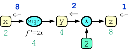
Recall that a computational graph is a sequence of operations used to obtain the value of some quantity. In machine learning, this is usually a scalar loss function (a zero-dimensional tensor). The result of computation is obtained during the forward pass through the graph. Below is a graph for the function $z = x\cdot x + \sin(2\cdot y)$ along with the node values (green color) at x=4 and y=3.14159265:

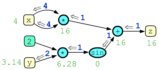
$$ z = x\cdot x + \sin(2\cdot y) $$ $$ \begin{array}{lcl} g_x = \frac{\displaystyle\partial z}{\displaystyle\partial x} &=& 2\cdot x\Bigr|_{x=4} = 8,\\[4mm] g_y = \frac{\displaystyle\partial z}{\displaystyle\partial y} &=& 2\,\cos(2\cdot y)\Bigr|_{y=\pi} = 2. \end{array} $$

After the forward pass through the graph (from the leaves to the root $z$ of the tree), the backward pass procedure is launched, which computes the derivatives (gradients, blue color) of the target expression $z$ with respect to other nodes in the graph. In the illustration, the node z outputs $g_z=1$. The total $g_x=8$ entering node x equals the partial derivative $\partial z/\partial x$, and $g_y=2$ entering y equals $\partial z/\partial y$. For more details on gradient computation, see the document "Computational Graph".

In PyTorch, graphs are dynamic. They are constructed during the execution of expressions. To repeat computations with new data, it is necessary to rebuild the entire set of operations. This approach differs from static graphs used in TensorFlow. A static graph is defined once, compiled, and can then be executed multiple times with different values in the leaf nodes, but cannot be modified.

Graph construction

A tensor in PyTorch, in addition to holding data values of its elements, can also store gradients of those elements and many other attributes necessary for working with a computational graph:

from torch import tensor, empty, ones, zeros

v  = zeros(2)                # 2D vector of zeros

print(v.data)                # tensor([0.,0.])  - tensor data (same as just v)
print(v.grad)                # None             - gradient of the tensor (not yet available)
print(v.grad_fn)             # None             - function that produced it (no graph yet)
print(v.is_leaf)             # True             - is a leaf node of the graph (yes)
print(v.requires_grad)       # False            - requires gradient (not yet)

All operations with the tensor v are performed using its attribute v.data. The attribute v.grad (if it exists) is a tensor of the same dimensionality as v (it also has data, grad,..., etc.).

In PyTorch, a graph begins to build if an expression includes a tensor with the attribute requires_grad set to True.
This attribute can be specified in the constructor (when creating the tensor) or at any later moment:

x = ones(2, requires_grad=True)          # vector [1., 1.] is immediately a graph node

y = empty(2).fill_(3)                    # first create vector [3.,3.],
y.requires_grad = True                   # then declare it as a graph node

print(y)                                 # tensor([3., 3.], requires_grad=True)

The attribute requires_grad is "contagious" - if at least one tensor in an expression has it set, a computational graph is created. Each of its non-leaf nodes stores the last operation that led to it (in the attribute grad_fn):

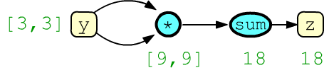
z = (y*y).sum()                          # scalar (dim=0) y[0]**2 + y[1]**2
 
print(z)                                 # tensor(18., grad_fn=<SumBackward0>)
print(y.is_leaf, z.is_leaf)              # True False
print(y.requires_grad, y.grad_fn)        # True None
print(z.requires_grad, z.grad_fn)        # True <SumBackward0>

The node y is a leaf (is_leaf), while z is not (it is the root = final node of the tree).

Gradient computation

The backward() method of the root node of a graph triggers the gradient computation procedure in the leaf (is_leaf) nodes that have the attribute requires_grad.
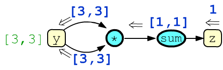
In the example above, the number 1, passing through the summation node, is duplicated as many times as there were summed elements, turning into a vector [1,1]. Then, at the elementwise multiplication node, it is multiplied by the opposite argument:

print(y.grad)                              # None
z.backward()                               # start gradient computation
print(y.grad)                              # tensor([6., 6.]) - sum of 2 incoming grads

The backward() method cannot be called again (only after rebuilding the graph). The exception is the following call: z.backward(retain_graph = True). However, in this case, the gradients will accumulate (sum up).

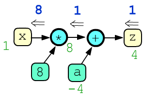Leaf nodes without the attribute requires_grad=True are treated as constants, and gradients are not computed for them. Below, there are two constants (8, a):

x = ones(1, requires_grad=True)
a = tensor(-4.)
z = 8*x + a

z.backward()

print(x, x.grad)         # tensor([1.], requires_grad=True), tensor([8.])
print(a, a.grad)         # tensor([-4.]), None
print(z)                 # tensor([4.], grad_fn=<AddBackward0>)

When analyzing the computation graph, it’s important to remember that any variable (leaf or intermediate) is always represented by a single node. If a variable is used in multiple computations, several edges will originate from it, and during backpropagation, several gradients will enter and be summed. Such was the case with node y in the example at the beginning of this section.

Gradient in intermediate nodes

By default, intermediate (non-leaf) nodes of the computation graph do not store the gradients that pass through them. This behavior can be changed
by calling the retain_grad method for a specific node:

x = tensor(2., requires_grad=True)

y  = x**2;    y.retain_grad()                    
z  = 2*y;     z.retain_grad()       

z.backward()

print(z.item(),     y.item(),     x.item())      # 8.0 4.0 2.0
print(z.grad.item(),y.grad.item(),x.grad.item()) # 1.0 2.0 8.0

In this example, the root of the computation tree is the tensor z, and the only leaf node requiring a gradient by default is x. The node y is an intermediate node.

Pausing graph construction

The computation graph must be rebuilt each time gradients are recalculated:

for i in range(1,3):
    x = empty(2).fill_(i).requires_grad_(True)
    
    z = x.dot(x)                           # graph
    z.backward()                           # compute gradients
    
    print(z.item(), x.grad)

In the loop above, a new tensor x is created twice, then a computation graph is built to calculate the sum of squares of its components: $z=x^2_0+x^2_1$. The gradient with respect to the leaf variable is: $\partial z/\partial x_i = 2x_i$.

Sometimes it’s necessary to perform operations on leaf nodes without modifying the computation graph. Such operations are performed within a no_grad context, which blocks the creation of new graph nodes. In the example below, memory for the tensor x is allocated only once (it's important for large tensors). Then, inside the no_grad block, the values in that memory are modified and the graph is built afterward. Since the leaf tensor x is not recreated, its gradients must be reset to prevent accumulation in subsequent loop iterations:

x = empty(2).requires_grad_(True)

for i in range(1,3):
    with torch.no_grad():                  # disabled gradient calculation
        x.fill_(i)                         # modify existing values 
        
    z = x.dot(x)
    z.backward()                           # computation graph
    
    print(z.item(), x.grad.numpy())    
    
    x.grad.zero_()                         # reset gradients

This and the previous example will produce the same results:

2.0  [2., 2.]
8.0  [4., 4.]

Another way to modify tensor data without affecting the computation graph is to work directly with its data attribute. For example, the above code could also be written as:

for i in range(1,3):
    x.data.fill_(i)                         # modify existing values 
...

After exiting the with block with torch.no_grad(), graph construction is automatically re-enabled. It can also be re-enabled manually using torch.enable_grad():

x = ones(1, requires_grad=True)
with torch.no_grad():                      # disable graph construction
    z1 = 2 * x
    with torch.enable_grad():              # enable graph construction 
        z2 = 2 * x
print(x.requires_grad, z1.requires_grad, z2.requires_grad)  # True False True

An example of iterative computations for finding optimal parameters of a linear model can be found in this document.

Detaching a node from the graph

Using the detach method, you can obtain a tensor that is "detached" from the computation graph - it will reference the data of the original node but will not be part of the graph:

x = tensor([1.,2.], requires_grad=True)   
y = x.detach()                                

print(x)                                   # tensor([1., 2.], requires_grad=True)
print(y)                                   # tensor([1., 2.])
y[0]=5 
print(x)                                   # tensor([5., 2.], requires_grad=True)

This is an alternative to using the no_grad() context for modifying leaf nodes without affecting the computation graph:

x  = empty(2).requires_grad_(True)
xd = x.detach()
 
for i in range(1,3):
    xd.fill_(i)
         
    z = x.dot(x)                   # start building the graph
    z.backward()                   # compute the gradient graph
     
    print(z.item(), x.grad)
     
    x.grad.zero_()                 # reset gradients

Some examples

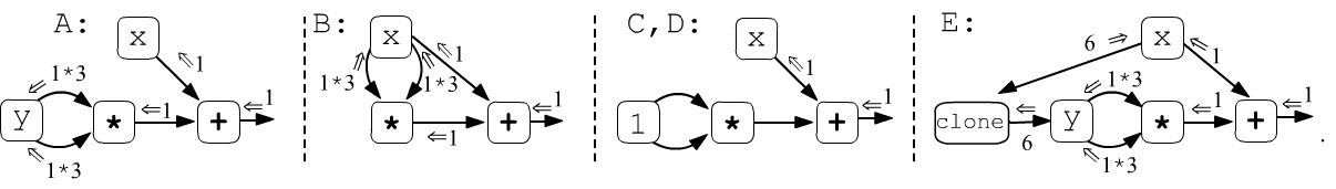
Let's look at an example where the forward pass produces the same value, but the gradients differ depending on how the variable y is formed:

x  = tensor(3.).requires_grad_(True)   #   x.grad y.grad  y.requires_grad
y  = tensor(3.).requires_grad_(True)   # A:  1    6       True  
#y = x                                 # B:  7    7       True  
#y = tensor(1.)                        # C:  1    None    False 
#y = x.detach().clone()                # D:  1    None    False
#y = x.clone()                         # E:  7    None    True, grad_fn=<CloneBackward>

z = x + y*y                            # z = 12
z.backward()

Case A: the derivatives are computed for two independent variables $z=z(x,y)=x+y^2$. This leads to the gradients: $\nabla_x\, z(x,y) = 1$ and $\nabla_y\, z(x,y) = 2y$.
Case B: the assignment y=x creates a reference, and y is simply another name for x. Thus, $z=z(x)=x+x^2$ and $\nabla_x\, z(x) = 1+2x$ (the gradient for y will be the same).
Cases C, D are equivalent. Using torch.tensor(1.) creates a tensor without requires_grad, so for the graph, it acts as a constant. Similarly, x.clone() creates a copy of x, which is then "detached" from the graph using detach (it later reconnects, but only as a constant).
Case E is a bit more complex and less meaningful. The x.clone() method creates a copy of x. This operation itself becomes a node in the graph. During the backward pass, two gradients (from addition and cloning) converge at the leaf node, and their sum gives 7.

In fact, cloning without detaching can sometimes lead to unexpected results, so when working within a computation graph, it’s generally better to use detach().clone() or perform the cloning within a no_grad context:

x = torch.ones(1, requires_grad=True)
                               # y.requires_grad:  y.grad_fn:
with torch.no_grad():          
    y = x.clone()              # False             None
y = x.detach().clone()         # False             None
y = x.clone()                  # True              <CloneBackward>

What not to do with graph leaves

In PyTorch, the starting (leaf) variables for which gradients are computed must not participate in in-place operations, nor can they be overwritten. Let’s take a closer look at these restrictions.

Recall that in-place operations modify the value of a variable without creating new memory. In PyTorch, all methods ending with an underscore are in-place operations: fill_(), add_(), mm_(), etc. In the example below, the last line performs a non-in-place operation (the result of x+1 is written into new memory — see the change in id()):

x = ones(1);    print(x, id(x))   # tensor([1.]) 2769629314008

x += 1;         print(x, id(x))   # tensor([2.]) 2769629314008   in-place
x.add_(1);      print(x, id(x))   # tensor([3.]) 2769629314008   in-place
x = x + 1;      print(x, id(x))   # tensor([4.]) 2769629311928   non in-place

The following code will raise an error: "a leaf Variable that requires grad has been used in an in-place operation":

x = tensor(1., requires_grad=True)
x += 1                             # in-place for leaf is not allowed!

The same error occurs in the code below (y is a reference to x, so this is effectively the same variable):

x = ones(1.,requires_grad=True); print(x,id(x)) # tensor(1.,requires_grad=True) ...95208
y = x                          ; print(y,id(y)) # tensor(1.,requires_grad=True) ...95208
y *= 1                                          # in-place on a leaf variable

For non-leaf nodes, in-place operations are allowed:

x = tensor(1.,requires_grad=True)   # x.grad = tensor(0.5)
y = 2*x                             # tensor(2.,     grad_fn=<MulBackward0>)
y += 2                              # tensor(4.,     grad_fn=<AddBackward0>)
y.log_()                            # tensor(1.3863, grad_fn=<LogBackward> )
y.backward()                        # y = log(2*x+2); y'=1/(x+1)

A leaf variable must not be reassigned, because doing so "destroys" it and causes it to lose the requires_grad property:

x = tensor(1., requires_grad=True) #  tensor(1., requires_grad=True)
x = x + 1                          #  tensor(2., grad_fn=<AddBackward0>) no requires_grad

Tensor slicing

Slices of tensors return a new tensor containing a portion of the original data. At the same time, they share the same underlying memory. Therefore, computing gradients in graphs involving slice operations requires some caution:

x = tensor(1., requires_grad=True)    
s = ones(2)
s[1] =  s[0] * x                      # s[1] =  s[0].clone() * x <- this is the correct way!
z = s.sum()                           # z = s[0] + s[0]*x
z.backward()

This code will raise the error: "one of the variables needed for gradient computation has been modified by an inplace operation". To fix it, you need to make a copy of the tensor element using s[1] = s[0].clone() * x. You must use the clone() method specifically: "Unlike copy_(), this function is recorded in the computation graph. Gradients propagating to the cloned tensor will propagate to the original tensor." In particular, in the graph the tensor s will have: s.grad_fn=<CopySlices>.

Assignment to a slice is an in-place operation, therefore it is prohibited for leaf variables. The following code will raise an error:

x, w = torch.randn(1), torch.randn(1, requires_grad=True)
w[0] = 1.
y = x*w
y.backward()

Finally, slices can significantly slow down the backward propagation of gradients. The two code examples below perform the same computation, but the one on the right runs almost 10 times slower:

y = []       
for i in range(100):
    x = torch.randn(1,256,256, 
                    requires_grad=True)
    y.append( x )        
y = torch.cat(y, dim=0)
z = y.sum()
z.backward()

y = torch.empty(100,256,256)        
for i in range(100):
    x = torch.randn(256,256, 
                    requires_grad=True)
    y[i] = x   
    
z = y.sum()
z.backward()

If you comment out z.backward(), the execution times become comparable.

Thus, when working with computation graphs, you should avoid slice assignments that lead to grad_fn=<CopySlices>.

Visualization

To visualize computation graphs, you can use a small library called torchviz (see its documentation and examples):

import torchviz
from torch import tensor, empty, ones, zeros

w, b = ones(5, requires_grad=True), tensor(0., requires_grad=True)
x = ones(5)
z = x.dot(w) + b

torchviz.make_dot(z,  params = {'x': x, 'w': w, 'b': b} )

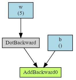
Note that the library only visualizes leaf nodes for which requires_grad=True is set.

Function minimization

Let’s look at an example of minimizing a multivariable function using the gradient method. For this, we’ll use the standard SGD optimizer:

import torch

def fun(x):    
    return x[0]**2 + (x[1]-1)**2

x = torch.tensor([1.,2.], requires_grad=True)    # initial values

optimizer = torch.optim.SGD([x],  lr=1, momentum=0.5) 
for it in range(20):
    optimizer.zero_grad()                        # reset gradients  
    y = fun(x)                                   # compute function value
    y.backward()                                 # compute gradients     
    optimizer.step()                             # update parameters
    
    print(y.item(), x.detach().numpy())