ML: Introduction to PyTorch: 1. Tensors
Introduction
 The PyTorch library is a versatile
machine learning tool.
It is popular for designing new neural network architectures.
It is an open-source project supported by Facebook.
The library has four key components:
The PyTorch library is a versatile
machine learning tool.
It is popular for designing new neural network architectures.
It is an open-source project supported by Facebook.
The library has four key components:
- An advanced toolkit for working with tensors. It is similar to numpy, but provides additional capabilities for memory allocation control, which is important when working with large models and datasets.
- Simple construction of a dynamic computational graph, allowing gradients of target functions with respect to model parameters to be obtained.
- A large set of ready-made layers for building neural networks of arbitrary architecture.
- The ability to redirect computations to graphics processors (GPU).
PyTorch must be installed by selecting the correct configuration on the project page and connecting the library:
import torch

e  = torch.eye(2)                    # 2x2 identity matrix
print(e)                             # tensor([[1., 0.],
                                               [0., 1.]])
To read this document, it is advisable to have a solid understanding of the numpy library, particularly such concepts as tensor dimensionality, its shape, and how they change during various operations. Below, we will review the basics of working with tensors. The following documents are devoted to computational graphs and neural networks in PyTorch.
Creating tensors
Tensors with real components of type float32 are created as follows:
v = torch.empty(10)                      # vector of 10 float32 elements (garbage)
m = torch.empty(2, 3)                    # matrix of shape (2,3) float32 (garbage)
x = torch.empty_like(m)                  # garbage, same shape as m
A tensor can also be created from a Python list or a numpy array:
x = torch.tensor( [ [0,1,2], [3,4,6] ] ) # matrix of shape (2,3) int64 from a list
s = torch.tensor(137.)                   # scalar (dim=0) of type float32 (note the dot!)
s = torch.tensor(137, dtype=torch.double)# same, but of type float64 (even without a dot)

e = torch.from_numpy( np.eye(3) )        # from a numpy tensor (shares its memory)

print( x )                               # tensor([[0., 1., 2.], [3., 4., 6.]])
print( x.numpy() )                       # numpy tensor (in the same memory)
The main properties of a tensor are its dimensionality (number of indices),
shape (dimensions of the indices), element type, and number of elements:
print( x.dim(),  x.type(), x.numel() )   # dimensionality, element type, element count
print( x.size(), x.shape )               # torch.Size([2, 3]) shape (equivalent)
print( tuple(x.shape), *x.shape )        # (2, 3) 2 3 shape

print( s.item(), s.dim()  )              # 137 0 (for a scalar or a matrix with one elem.)
A tensor can also be created using constructors. The following types are available (instead of torch.FloatTensor(...) you can write torch.Tensor(...)):
   HalfTensor   - float16,      ShortTensor - int16,        CharTensor - int8,
   FloatTensor  - float32,      IntTensor   - int32,        ByteTensor - uint8,
   DoubleTensor - float64,      LongTensor  - int64,        BoolTensor - bool.
When changing the data type (if it changes), new memory is allocated for the data:
x = torch.Tensor(2,3)                    # matrix (2,3) of 6 float32 elements (garbage)
y = x.long()                             # int64   new tensor
y = x.float()                            # float32 new tensor
y = x.double()                           # float64 new tensor
The element type can also be specified in the empty method or in initialization functions (see below):
x = torch.empty(2,3, dtype=torch.float64)# 2x3 matrix with garbage float64
x = torch.empty(2,3, dtype=torch.double) # same thing
y = torch.zeros(2,3, dtype=torch.int64)  # 2x3 matrix of zeros int64
y = torch.zeros(2,3, dtype=torch.long)   # same thing

y.element_size()                         # 8 - size in bytes of each element
Value initialization
When creating a tensor, you can immediately initialize its values (by default of type float == float32):
y = torch.zeros (2, 3)                   # 2x3 matrix of zeros, type float32
x = torch.zeros_like(y)                  # same shape as y, filled with zeros

x = torch.ones (2, 3)                    # 2x3 matrix of ones
x = torch.ones_like(y)                   # same shape as y, filled with ones

x = torch.full((2, 3), 3.14159265)       # fill 2x3 matrix with the number pi

x = torch.eye   (3)                      # 3x3 identity matrix
x = torch.eye   (2,3)                    # "identity" non-square matrix [[1., 0., 0.],
                                         #                               [0., 1., 0.]]
x = torch.linspace(0,2,5)                # [0.0,0.5,1.0,1.5,2.0] [beg,end], num

x = torch.rand (2, 3)                    # 2x3 uniform random matrix [0...1]
x = torch.randn(2, 3)                    # 2x3 normal random matrix (mean=0, var=1)

x = torch.empty(3).uniform_(0, 1)        # vector with uniform distribution [0..1]
x = torch.empty(3).normal_(mean=0,std=1) # vector with normal distribution
The following methods by default return elements of type long == int64:
x = torch.arange(4)                      # [0,1,2,3]             [0,end)
x = torch.arange(2,14,3)                 # [2,5,8,11]            [beg,end), step

x = torch.randperm(10)                   # [8,6,9,3,5,0,1,4,7,2] - random permutation
x = torch.randint (1, 10, (2,3))         # 2x3 random integers from interval [1...10)
Memory management
Many methods have a second version whose name ends with an underscore (in-place functions). For example, taking the exponential of a tensor’s elements: x.exp() or torch.exp(x) returns a new tensor. The method x.exp_() computes the exponential of the elements of x and writes the results into the same memory locations, i.e., no new memory is allocated (the item() method returns a single tensor element as a number):
x = torch.ones(1)                        # vector with one component
y = x.exp()                              # different memory:
print(x); y[0]=2;  print(x.item())       # tensor([1.])      1.0

y = x.exp_()                             # same memory:
print(x);  y[0]=2;  print(x.item())      # tensor([2.7183])  2.0
The same semantics apply to the fill_ method, which assigns a given value to all elements, and to the zero_ method, which sets all elements to zero:
x = torch.empty(2, 3).fill_(-1)          # matrix filled with -1
x.zero_()                                # now zeros (in the same tensor)
The assignment operator, as usual, works by reference (data is shared). If a data copy is needed, it can be obtained using the clone or copy_ method:
y = x                                    # y and x are the same object
y = x.clone()                            # copying

y.copy_(x)                               # copies x into itself (broadcastable)
y = torch.empty_like(x).copy_(x)         # allocate memory and copy
For "regular" tensors, copy_ and clone produce the same result. The difference appears when constructing the computation graph (see below).
Operations
Most tensor operations are the same as in the numpy library:
x1, x2 = torch.ones(2,3),  torch.ones(2,3)

x1[0]   = 2           # change the first row to 2     [ [2., 2., 2.],  [1., 1., 1.]]
x2[:,1] = 3           # change the second column to 3 [ [1., 3., 1.],  [1., 3., 1.]]

y = x1 + x2           # addition                      [ [3., 5., 3.],  [2., 4., 2.]]
Addition, subtraction, multiplication, and division (without reduction) can be performed incrementally (in-place):
x += y
x.add_(y)             # add y to tensor x (increment)
x.add_(y, alpha=2.0)  # x += 2*y (faster for large tensors)

x *= y
x.mul_(y)
Using an index tensor, you can select specific elements:
a = torch.ByteTensor(2,3).random_() # random bytes [[185,  16, 242], [223, 147, 202]]

print(a > 128)                      # [[ True, False,  True], [ True,  True,  True]]
a[a > 128]                          # [185, 242, 223, 147, 202] - elements greater than 128
A useful example of such operations is synchronized shuffling of tensors (new memory is created):
X = torch.arange(10)                # [ 0, 1, 2, 3, 4, 5, 6, 7, 8, 9]
Y = -X                              # [ 0,-1,-2,-3,-4,-5,-6,-7,-8,-9]

idx = torch.randperm(X.shape[0])    # index permutation
X = X[idx]                          # [ 4, 9, 7, 3, 2, 0, 5, 6, 1, 8]
Y = Y[idx]                          # [-4,-9,-7,-3,-2, 0,-5,-6,-1,-8]
Tensors can be concatenated along a specific axis or stacked:
x1 = torch.arange(-3,0)             # [-3, -2, -1]
x2 = torch.arange(3)                # [ 0,  1,  2]

torch.cat([x1, x2], dim=0)          #  [-3, -2, -1,  0,  1,  2]    concatenation
torch.stack([x1, x2])               # [[-3, -2, -1], [ 0,  1,  2]]
Tensor convolutions
All functions in this section exist in two equivalent versions: x.mm(y) and torch.mm(x,y).
v.dot(u)                # scalar multiplication - only for 1D vectors
x.mv(v)                 # matrix-vector multiplication: (n,s) (s)   = (n)
x.mm(y)                 # only for 2D matrices: (n,s) (s,m) = (n,m)

x.bmm(y)                # for 3D tensors:   (b, n,s) (b, s,m) =   (b, n,m)
x.matmul(y)             # numpy equivalent: (j,1, n,s) (k, s,m) = (j,k, n,m)

torch.addmv(t, m, v, beta=1, alpha=1)  #  alpha*(m  @ v)  + beta*t
torch.addmm(t,m1,m2, beta=1, alpha=1)  #  alpha*(m1 @ m2) + beta*t
Many functions perform calculations either across all elements or along one of the indices (along an axis). Below, the axis is 1 (the second index):
x = torch.Tensor([[2,1,3],
                  [1,2,1]])
x.sum(1)                # [6., 4.]   sum
x.mean(1)               # [2., 1.33] mean
x.prod(1)               # [6., 2.]   product

x.argmin(1)             # [1, 2]

v,i = x.topk(2, dim=1)  # 2 largest values and their indices
Similarly: std(), var(), median(), max(), min().
Reshaping
The shape of a tensor (the number of indices and their dimensions) can be changed using the functions view and reshape:
torch.arange(6).view(2,3)         #    tensor([[0, 1, 2],
torch.arange(6).reshape(2,3)      #            [3, 4, 5]])
In these functions, new dimensions are specified (their product must match the total number of elements). One of the dimensions can be set to -1, and it will be calculated automatically. For example, the above could also be written as view(-1,3) or view(2,-1). You can also reshape a tensor using another tensor with the same number of elements:
a, b = torch.zeros(2,5), torch.zeros(10)
b.view_as(a)
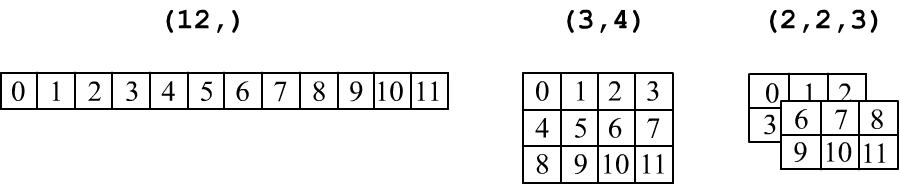
Recall that tensors are commonly represented in tabular form: a vector (ndim=1) is a row of numbers, a matrix of shape (rows, cols) is a rectangular table with rows and columns. A three-dimensional tensor (three indices, ndim=3) is represented as a stack of matrices:
The transposition operation (swapping rows and columns): t() or t_() is allowed only for 2D matrices:
z = x.t()                              # x itself does not change
z = x.t_()                             # x is modified
Swapping any two axes (indices) in tensors of arbitrary dimensions is done using the transpose method:
x.transpose(1, 2) # swap axes 1 and 2Remember that x.t() is not the same as x.view(x.shape[1], x.shape[0]).
An even more general way to permute indices:
x = torch.randn(3, 5)
x.permute(1, 0) == x.t()               # equivalent to transposition

x = torch.randn(2, 3, 5)
x.permute(2, 0, 1).size()              # torch.Size([5, 2, 3])
Elements in memory
The shape of a tensor (x.size() or x.shape) is the way to number linearly ordered tensor elements using x.dim() indices. The method x.stride() provides a set of offsets by which indices are multiplied to obtain the corresponding element (from the pointer to the beginning):
x[i,j,k] = x + stride[0]*i  #  shape[1]*shape[0]
             + stride[1]*j  #  shape[0]
             + stride[2]*k  #  1                          (pseudocode)
For example:
x = torch.arange(935).view(5,17,11)    #     11*17
print( x.stride(), x[1,1,1].item() )   #< (187, 11, 1) 199=187+11+1
When the shape changes using view, the x.stride() changes, but not the data in memory. However, this may cause a situation where the rows of the matrix are not stored consecutively in memory. In the figure below, tensor x is a 2D matrix of shape (2,3). Its elements are stored in memory sequentially, row by row. The transposition operation (without an underscore) does not modify the original tensor and returns a reference to the same data but with a different stride. As a result, its rows appear “scrambled” in memory. If you call the y.contiguous() method, a new memory block will be created, and the elements will be rearranged so that rows follow each other sequentially:

You can check whether the tensor rows are stored consecutively in memory as follows:
print( x.is_contiguous() ) # True - continuous row-wiseFor arbitrary dimensions, this method checks the condition stride[i]=stride[i+1]*size[i+1] for all indices. If this condition is not met, the x = x.contiguous() method can move the data into a continuous memory block.
When changing the shape using reshape, it first checks is_contiguous, and if it is False, it calls contiguous (creating new memory). After that, view is invoked. Thus, in the example in the figure, for the operation y=x.t(), the tensors x,y share the same data (by reference), but after y = y.contiguous() they no longer do.
Therefore, reshape may return data either by reference or by value. The view method always returns by value, but may raise an error if the is_contiguous condition is violated.
GPU computing
Let's multiply two large identity matrices. On a central processor Intel i3-3220 3.3GHz, 16Gb this will take 35 seconds:x1 = torch.eye(10000) y1 = torch.eye(10000) z1 = x1.mm(y1) # 35sIf the computer has a graphics card (for example, NVIDIA GeForce GTX 1050 Ti), you can create an additional computational device (zero indicates the GPU index):
torch.cuda.device_count()              # number of available GPUs

cpu = torch.device("cpu")
gpu = torch.device("cuda:0" if torch.cuda.is_available() else "cpu")
Let’s repeat the same calculations by creating and multiplying tensors directly on the GPU:
x1 = torch.eye(10000, device = gpu)
y1 = torch.eye(10000, device = gpu)
z1 = x1.mm(y1)                         # 0.04s
In practice, tensors are often created in CPU memory, then transferred to the GPU using the to method, multiplied there, and finally moved back to the CPU:
x1 = torch.eye(10000).to(gpu)
y1 = torch.eye(10000).to(gpu)
z1 = x1.mm(y1).to(cpu)                 # 2s
You can check the amount of GPU memory currently in use as follows:
from GPUtil import showUtilization as gpu_usage
gpu_usage()
Sometimes, it needs to be cleared manually:
torch.cuda.empty_cache()Useful articles on GPU computing:
- PyTorch 101, Part 4: Memory Management and Using Multiple GPUs
- Use GPU in your PyTorch code;
- Speed Up your Algorithms Part 1 — PyTorch
