ML: Computational Graph

Introduction
General statement of the problem
Spoiler
Forward and backward passes
Derivatives for scalars
Gradients for tensors

Graph for composite functions
Addition and multiplication of tensors
Tensor convolutions
Tensor functions
Softmax and cross-entropy loss
Mini-PyTorch

Introduction

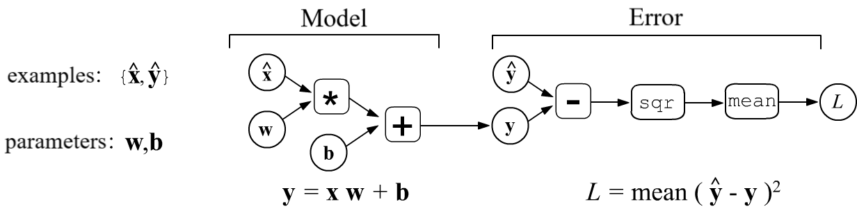
Machine learning is typically reduced to minimizing a scalar function that depends on a set of variables. The simplest example is the linear model, which is represented by the equation $\mathbf{y} = \mathbf{x}\cdot\mathbf{w} + \mathbf{b}$, where $\mathbf{w}$ (matrix) and $\mathbf{b}$ (vector) are the model parameters.
The training error $L$ is computed based on a set of training examples $\{\hat{\mathbf{x}},\hat{\mathbf{y}}\}$. For the mean squared error (MSE), it is equal to the average of the squared differences between the training values $\hat{\mathbf{y}}$ and the model outputs $\mathbf{y}$:

The model error depends on its parameters $L=L(\mathbf{w},\mathbf{b})$. Training the model involves searching for parameter values that minimize the error: $\mathbf{w},\,\mathbf{b} = \text{argmin}\,L(\mathbf{w},\,\mathbf{b})$. If there are many parameters, the most effective method is the gradient method and its various modifications. For a complex model, it is not easy to analytically calculate the gradient (derivatives with respect to the parameters). It is more convenient to represent the model as a computational graph. The graph has the topology of a tree. The root of the tree is the desired quantity (the error $L$), and he nodes perform elementary calculations. If the derivatives at each node are known, then the error gradient can also be found from the model parameters that are in the leaves of the tree. This approach is the basis of all modern machine learning frameworks.

General statement of the problem

Let the model be given by the function $\mathbf{y}=f(\mathbf{x},\,\mathbf{p})$, where $\mathbf{x}$ is a feature vector of an object, and $\mathbf{p}$ is a vector of parameters.
In addition, there are $N$ training examples $\{\hat{\mathbf{x}},\,\hat{\mathbf{y}}\}=(\hat{\mathbf{x}}^{(1)},\,\hat{\mathbf{y}}^{(1)}),\,...,\,(\hat{\mathbf{x}}^{(N)},\,\hat{\mathbf{y}}^{(N)})$, which are marked with a hat.
The parameters $\mathbf{p}$ of the model are adjusted to minimize the mean error $L$ for one example: $$ L ~=~ L(\mathbf{p})~=~ \frac{1}{N}\sum^N_{i=1} L(\hat{\mathbf{y}}^{(i)},\,\mathbf{y}^{(i)}),~~~~~~~~~~~ \mathbf{y}^{(i)} = f(\hat{\mathbf{x}}^{(i)},\mathbf{p}). $$ To find the minimum of $L$, it is necessary to shift the vector of parameters in the direction opposite to the gradient (partial derivatives) of $L$ with respect to $\mathbf{p}$. The shift value is determined by the scalar hyperparameter $\lambda$ (learning rate):

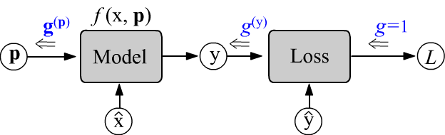
$$ \mathbf{p}\mapsto \mathbf{p} - \lambda\,\mathbf{g},~~~~~~~~~~~~~~~~\mathbf{g}= \frac{\partial L}{\partial \mathbf{p}}. $$

Computations are performed in two stages. First, during the forward pass (left-to-right), the error $L$ is computed with given $\hat{\mathbf{x}}$, $\hat{\mathbf{y}}$ and $\mathbf{p}$. At this stage, all nodes of the computational graph take on defined values.
Then the backward pass procedure is initiated. The initial gradient $g$ at the scalar node of error $L$ is a scalar. Passing through the nodes of the graph from the error from right to left, it is transformed into a vector $\mathbf{g}$ (generally into a tensor). The changes in $\mathbf{g}$ at each node occur in such a way that when it "reaches" the parameters $\mathbf{p}$, it turns out to be equal to the partial derivatives: $\mathbf{g}^{(\mathbf{p})}=\partial L/\partial\mathbf{p}$.

Forward and backward passes

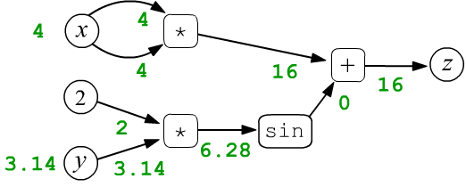
Let's consider the function $z=f(x,y)=x\cdot x + \sin(2 y)$ as a simple example of a function with two scalar variables $x$ and $y$. Let $x=4$ and $y=3.14159$. These numbers are assigned to the leaf nodes $x,y$ and then they are propagated through the computational graph from left to right. So, the multiplication node includes two arrows of each argument of the operation. In the first such node, they "carry" the same values $4$, which, when multiplied, gives the output value of $16$ (green color). As a result, each node, including the final one ($z=16$), takes on a certain value:

$$ z = x\cdot x + \sin(2\cdot y) $$

After the forward pass through the graph, the backward propagation of derivatives is launched. In the figure below, a number $g_z$ (which is assumed to be equal to $1$) emerges from the root node $z$. It moves through the graph towards the leaf nodes $x,y$. As it passes through each node, its value changes in a certain way:

$$ \begin{array}{lcl} g_x = \frac{\displaystyle\partial z}{\displaystyle\partial x} &=& 2\cdot x,\\[4mm] g_y = \frac{\displaystyle\partial z}{\displaystyle\partial y} &=& 2\,\cos(2\cdot y) \end{array} $$

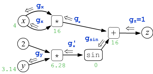
It is necessary to determine the rules of these changes in such a way that the values $g_x, g_y$ included in the leaf nodes $x,y$ turn out to be the partial derivatives of $z$ with respect to $x,y$.

Spoiler

This document contains many complex formulas. To avoid getting lost in them, let's first list the main rules of backpropagation:

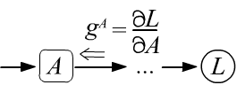
The gradient $g^A$ entering any node $A$, corresponds to the derivative of the target variable (the root of the tree) with respect to the value at this node: $g^A = \partial L/\partial A$.
The tensor dimension of the gradient entering a node is the same as the dimension of the tensor produced by this node on its output.
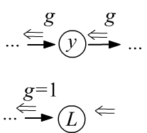
The gradient passes through variable nodes without changes, and "does not enter" constant nodes.
The initial gradient entering and exiting the root of the tree $L$ is equal to one,
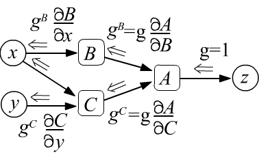
since by definition it is: $g=\partial L/\partial L =1$.
After passing through a node, the gradient is split along all the edges entering the node and multiplied by the derivatives between the nodes that the edge connects (see the left figure below).
If multiple gradients enter a node, they are summed (see the right figure below), which is a consequence of the rule for computing the derivative of a composite function (formula under the figure).

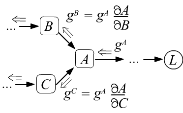$$ g^B ~=~ \frac{\partial L}{\partial B} ~=~ \frac{\partial L}{\partial A}\,\frac{\partial A}{\partial B} ~=~ g^A\,\frac{\partial A}{\partial B}, $$

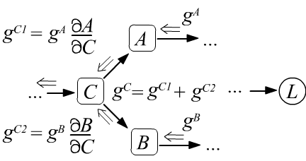$$ g^C ~=~ \frac{\partial L}{\partial C} ~=~ \frac{\partial L}{\partial A}\,\frac{\partial A}{\partial C} + \frac{\partial L}{\partial B}\,\frac{\partial B}{\partial C} ~=~ g^A\,\frac{\partial A}{\partial C} + g^B\,\frac{\partial A}{\partial B}. $$

Derivatives for scalars

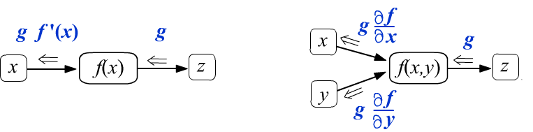
Let's first consider scalar functions of one $f(x)$ and two $f(x,y)$ variables. Nodes that compute them have one and two edges respectively (function arguments). Let's assume that during backpropagation, some number $g$ enters the function node from right to left. We require that it changes as follows at the output:

(def1)

When passing through a node that computes $f(x)$, the value $g$ is multiplied by the derivative of the function $f'(x)$. The analytical expression for $f'(x)$ is known, since it is assumed that the function of a computational graph node is sufficiently simple.
The numerical values of $f(x)$ and $f'(x)$ depend on the value of the argument $x$, which is known as a result of the forward pass through the graph (from left to right). A similar situation holds for a function of two variables.

If the graph consists only of these nodes, then with the initial gradient $g=1$, we obtain correct expressions for the derivatives entering the leaf nodes $x,y$.

Let's apply these definitions to the sine function and to the operations of addition and multiplication:

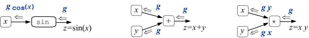
Thus, the addition operation does not change the gradient $g$ passing through it, splitting it into two identical values. When passing through a multiplication node, the gradient changes by being multiplied by the "other" argument.

Now it is easy to write the propagation of derivatives for the function $z=x*x+\sin(2*y)$:

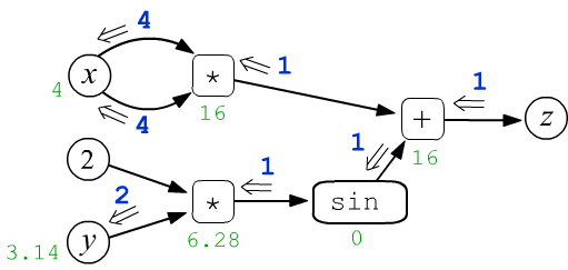
taking into account that $\cos(2\pi)=1$. Thus, a value of two enters the node $y$ ($\partial z/\partial y = 2$), and the node $x$ receives four twice, i.e. $\partial z/\partial x = 8$.

Here is an example of computing these gradients in PyTorch:

from torch import tensor, sin

x, y = tensor(4., requires_grad=True), tensor(3.14159265, requires_grad=True)

z = x*x + sin(2*y)    # graph with root: tensor(16., grad_fn=<AddBackward0>)

z.backward()          # start gradient computation (the backward pass)

print(x.grad, y.grad) # tensor(8.)  tensor(2.)

In this Python code, two tensors $x,y$ of zero dimension (scalars) are introduced. The property requires_grad means that these tensors will be the leaves of the computation tree. As the expression for $z$ (the root) is written, this tree is constructed directly, and at the same time the forward pass is executed (the value of $z$ is computed). Calling the backward method initiates the backward pass, as a result of which $x$ and $y$ obtain the grad property containing the values of the derivatives $\partial z/\partial x$ and $\partial z/\partial y$.

Graph for composite functions

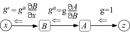
Consider as an example the backpropagation for composite functions. Below on the left, $z$ is equal to function $A$, which depends on function $B(x)$. The derivative of $z$ with respect to $x$ is taken as the derivative of a composite function (the formula under the figure). We arrive at the same result by analyzing backpropagation of the derivative through the graph. A one exits node $z$. Entering node $B$ it becomes $\partial A/\partial B$. After passing through node $B$, this derivative is multiplied by $\partial B/\partial x$:

$$ z = A(\,B(x)\,) $$

$$ g^x ~=~ \frac{\partial z}{\partial x} ~=~ \frac{\partial A}{\partial x} ~=~ \frac{\partial A}{\partial B}\,\frac{\partial B}{\partial x}, $$

$$ z = A(\,B(x),\,C(x,y)\,) $$

$$ g^x ~=~ \frac{\partial z}{\partial x} ~=~ \frac{\partial A}{\partial x} ~=~ \frac{\partial A}{\partial B}\,\frac{\partial B}{\partial x} ~+~ \frac{\partial A}{\partial C}\,\frac{\partial C}{\partial x}. $$

The second example is analyzed in a similar way. In it, the gradient flow splits at node $A$, and then converges at leaf $x$. These two derivatives must be summed, which corresponds to the plus sign in the partial derivative formula (under the figure).

Gradients for tensors

In machine learning tasks, the root of the graph (tree) is usually a scalar value (for example, the model error), while the leaf nodes of the graph (the model parameters) are tensors. The partial derivatives of the root with respect to the components of the tensor are precisely what are called gradients.

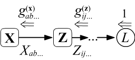Let a gradient from the scalar loss function $L$ enter the model. It propagates through the graph and enters some node $\mathbf{Z}$ from the right in the form of a tensor $g^{(\mathbf{Z})}_{ij...}$. In this node a computation occurs that transforms the tensor into $g^{(\mathbf{X})}_{\alpha\beta...}$ and it enters node $\mathbf{X}$.

Depending on the nature of the computation in $Z$, the number of indices and tensor dimensionality may change. At the same time, the dimensionality and shape of the gradient entering the node must always match the dimensionality and shape of the data stored in that node. Since $L$ depends on tensor $\mathbf{Z}$, which depends on tensor $\mathbf{X}$, the derivative of the composite function is computed as follows:

$$ g^{(\mathbf{X})}_{\alpha\beta...} ~=~ \frac{\partial L}{\partial X_{\alpha\beta...}} ~=~ \sum_{i,j,...} \frac{\partial L}{\partial Z_{ij...}}~\frac{\partial Z_{ij...}}{\partial X_{\alpha\beta...}} ~=~ \sum_{i,j,...} g^{(\mathbf{Z})}_{ij...}~\frac{\partial Z_{ij...}}{\partial X_{\alpha\beta...}}. $$

(def2)

If the root of the computational graph is a scalar value, then the gradient leaving it, as before, is set equal to 1, since $\partial L / \partial L = 1$.

☯ The definition above can be generalized to the case when the root of the graph is a tensor rather than a scalar. Depending on the goals, the gradient in it is initialized by one tensor or another (with the same dimensionality!). For example, if this tensor consists of ones: $g^{(\mathbf{L})}_{ij...}=g^{(\mathbf{Z})}_{ij...}=1$, then all components of the root tensor will be summed, which will turn it into a scalar:

$$ g^{(\mathbf{X})}_{\alpha\beta...} ~=~ \sum_{i,j,...} \frac{\partial Z_{ij...}}{\partial X_{\alpha\beta...}} ~=~ \frac{\partial Z}{\partial X_{\alpha\beta...}},~~~~~~~~~~~~~~~Z~=~\sum_{i,j,...} \,Z_{ij...} $$

To obtain the partial derivative directly with respect to the components $Z_{ij...}$, one must take $g^{(\mathbf{Z})}_{ij...}$ consisting of zeros except for a single element with indices $i,j,...$ equal to one (a projection tensor). However, for machine learning these cases are not important.

Addition and multiplication of tensors

Before analyzing how gradients propagate through different computational nodes, it is useful to review how the Kronecker symbol $\delta_{ij}$ is used (see the corresponding reminder in this document).

✒ The simplest node adds two tensors with the same number of indices. Using definition (def2), we have:

$$ Z_{ij...} = X_{ij...} + Y_{ij...}, ~~~~~~~~~~~~~ g^{(\mathbf{X})}_{\alpha\beta...} ~=~ \sum_{ij...} g^{(\mathbf{Z})}_{ij...}\,\frac{\partial Z_{ij...}}{\partial X_{\alpha\beta...}} ~=~ \sum_{ij...} g^{(\mathbf{Z})}_{ij...}\,\delta_{i\alpha}\,\delta_{j\beta}... ~=~ g^{(\mathbf{Z})}_{\alpha\beta...} $$

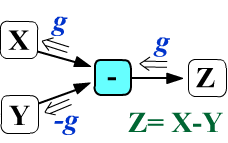This shows that addition does not change the gradient: it simply splits it into two identical tensors that are passed into the nodes of both operands. For subtraction $Z_{ij...} = X_{ij...} - Y_{ij...}$, the gradient entering node Y changes its sign, while the gradient entering X remains unchanged.

✒ If $\mathbf{M}$ is a matrix of shape (n,m) and $\mathbf{v}$ is a vector with m components, then their addition triggers broadcasting of vector $\mathbf{v}$: (n,m)+(m,) = (n,m)+(1,m) = (n,m). In this case, the gradient $\mathbf{g}^{(\mathbf{v})}$ entering the vector argument node $\mathbf{v}$ is also a vector:

$$ Z_{ij} = M_{ij} + v_j, ~~~~~~~~~~~~~~~~~ g^{(\mathbf{v})}_{\alpha} = \sum_{i,j} g^{(\mathbf{Z})}_{ij}~\frac{\partial Z_{ij}}{\partial v_{\alpha}} ~=~ \sum_{i,j} g^{(\mathbf{Z})}_{ij}~\delta_{j\alpha} ~=~ \sum_i \,g^{(\mathbf{Z})}_{i\alpha}. $$

The matrix argument $M_{ij}$ receives the gradient $g^{(\mathbf{Z})}_{ij}$ unchanged. In general, summation for the gradient is performed over all indices that were subject to broadcasting.

✒ Consider a node that multiplies tensors (without contraction). For example, two matrices:

$$ Z_{ij} = M_{ij}\,N_{ij},~~~~~~~~~~~~~~~ g^{(\mathbf{M})}_{\alpha\beta} = \displaystyle\sum_{ i,j} g^{(\mathbf{Z})}_{ij}~\frac{\partial Z_{ij}}{\partial M_{\alpha\beta}} = \displaystyle\sum_{i,j} g^{(\mathbf{Z})}_{ij}~\delta_{i\alpha}\delta_{i\beta}\, N_{ij} = \displaystyle g^{(\mathbf{Z})}_{\alpha \beta}\, N^{\phantom{(\mathbf{Z})}}_{\alpha\beta} $$

and similarly for $g^{(\mathbf{N})}_{\alpha\beta}$ Thus, the gradient transformation mirrors the familiar scalar case: when passing through a product node, each gradient is multiplied by the other operand.

Tensor convolutions

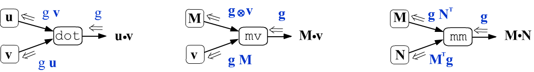
✒ Let's consider the convolution of two vectors at the dot node. Its result will be a scalar, so the scalar $g^{(z)}$ enters the node:

$$ z = \sum_i u_i\,v_i,~~~~~~~~~~~~~~ g^{(\mathbf{u})}_\alpha = g^{(z)}\, \displaystyle\frac{\partial z}{\partial u_{\alpha}} = g^{(z)}\,v_{\alpha}, $$

and similarly for $g^{(\mathbf{v})}_{\alpha} $ Thus, during backpropagation, the scalar $g^{(z)}$ enters the dot node, and upon exiting it transforms into two vectors: $\mathbf{g}^{(\mathbf{u})} = \mathbf{g}^{(z)} \, \mathbf{v}$ and $\mathbf{g}^{(\mathbf{v})} = \mathbf{g}^{(z)} \, \mathbf{u}$.

✒ Convolution of a matrix $M_{ij}$ and a vector $v_j$ in the PyTorch framework is denoted as mv.
The result of the operation is a vector, so the gradient entering the node is also a vector $g^{(\mathbf{z})}_{i}$:

$$ z_i = \sum_{j} M_{ij}\,v_{j},~~~~~~~~~~~~~~~ \left\{ \begin{array}{lclclcl} g^{(\mathbf{M})}_{\alpha\beta} &=& \displaystyle\sum_{ i} g^{(\mathbf{z})}_{i}~\frac{\partial z_{i}}{\partial M_{\alpha\beta}} &=& \displaystyle\sum_{i,j} g^{(\mathbf{z})}_{i}~\delta_{i\alpha}\delta_{j\beta}\, v_j &=& \displaystyle g^{(\mathbf{z})}_{\alpha}\, v_\beta,\\[3mm] g^{(\mathbf{v})}_{\alpha} &=& \displaystyle\sum_{i} g^{(\mathbf{z})}_{i}~\frac{\partial z_{i}}{\partial v_{\alpha}} &=& \displaystyle \sum_{i,j} g^{(\mathbf{z})}_{i}~M_{ij}\,\delta_{j\alpha} &=& \displaystyle \sum_{i} g^{(\mathbf{z})}_{i}~M_{i\alpha}. \end{array} \right. $$ The product of the components of the two vectors $g^{(\mathbf{z})}_{\alpha}\, v_\beta$ is called the outer product: $\mathbf{g}^{(\mathbf{M})}=\mathbf{g}^{(\mathbf{z})}\otimes \mathbf{v}$ (a matrix).
The second formula is just a matrix-vector convolution: $\mathbf{g}^{(\mathbf{v})} = \mathbf{g}^{(\mathbf{z})}\,\mathbf{M}$.

✒ Computation for the convolution of two matrices (resulting in a matrix again) is carried out similarly:

$$ Z_{ij} = \sum_{k} M_{ik}\,N_{kj},~~~~~~~~~~~~~~~ \left\{ \begin{array}{lclclcl} g^{(\mathbf{M})}_{\alpha\beta} &=& \displaystyle\sum_{ i,j} g^{(\mathbf{Z})}_{ij}~\frac{\partial Z_{ij}}{\partial M_{\alpha\beta}} &=& \displaystyle\sum_{i,j,k} g^{(\mathbf{Z})}_{ij}~\delta_{i\alpha}\delta_{k\beta}\, N_{kj} &=& \displaystyle\sum_{j} \displaystyle g^{(\mathbf{Z})}_{\alpha j}\, N^{\phantom{(\mathbf{Z})}}_{\beta j}, \\[3mm] g^{(\mathbf{N})}_{\alpha\beta} &=& \displaystyle\sum_{i,j} g^{(\mathbf{Z})}_{ij}~\frac{\partial Z_{ij}}{\partial N_{\alpha\beta}} &=& \displaystyle \sum_{i,j,k} g^{(\mathbf{Z})}_{ij}~M_{ik}\,\delta_{k\alpha}\delta_{j\beta} &=& \displaystyle \sum_{i} M^{\phantom{(\mathbf{Z})}}_{i\alpha}\,g^{(\mathbf{Z})}_{i\beta}. \end{array} \right. $$ By swapping indices in the matrix using the transpose operation $M^\top_{\alpha\beta}=M_{\beta\alpha}$, these formulas can be written in index-free form: $~~\mathbf{g}^{(\mathbf{M})}= \mathbf{g}^{(\mathbf{Z})}\,\mathbf{N}^\top~~$ and $~~\mathbf{g}^{(\mathbf{N})}= \mathbf{M}^\top\,\mathbf{g}^{(\mathbf{Z})}$.

We can represent the above formulas graphically, omitting indices for matrices and vectors:

Example of computing the gradient for the scalar product of two vectors $z=\mathbf{u}\cdot \mathbf{v}$, for which $\partial z/\partial \mathbf{u} = \mathbf{v}$:

u, v = tensor([1.,2.], requires_grad=True), tensor([3.,4.], requires_grad=True)

z = u.dot(v)         # tensor(11., grad_fn=<DotBackward>)

z.backward()          # perform gradient computation

print(u.grad)         # tensor([3., 4.])
print(v.grad)         # tensor([1., 2.])

Tensor functions

Let's now consider functions of a tensor. If it is a "regular" function applied independently to each element of the tensor, then everything works as in the scalar case:

$$ Z_{ij...} = f(X_{ij...}),~~~~~~~~~~ g^{(\mathbf{X})}_{\alpha\beta...} ~=~ \sum_{i,j,...} g^{(\mathbf{Z})}_{ij...}~\frac{\partial f(X_{ij...})}{\partial X_{\alpha\beta...}} ~=~\sum_{i,j,...} g^{(\mathbf{Z})}_{ij...}~f'(X_{ij...})~\delta_{i\alpha}\delta_{j\beta}... ~=~ g^{(\mathbf{Z})}_{\alpha\beta...}~f'(X_{\alpha\beta...}). $$ The most popular functions in neural networks have the following derivatives: $$ \left\{ \begin{array}{rcl} y=\sigma(x)&=&\displaystyle\frac{1}{1+e^{-x}},\\[3mm] \sigma'(x)&=& y\,(1-y) \end{array} \right. ~~~~~~~~~~~~~ \left\{ \begin{array}{rcl} y=\tanh(x) &=& \displaystyle\frac{e^{x}-e^{-x}}{e^{x}+e^{-x}}\\[3mm] \tanh'(x) &=& 1-y^2 \end{array} \right. ~~~~~~~~~~~~~ \left\{ \begin{array}{rcl} y=\text{relu}(x) &=& \text{max}(0,\,x)\\[3mm] \text{relu}'(x) &=& \mathrm{0~if~x~<~0~else~1} \end{array} \right. $$

It is slightly more complicated for functions that change the tensor's shape. For example, consider summing a tensor along the first index: X.sum(axis=0):

$$ Z_{jk...} = \sum_i X_{ijk...},~~~~~~~~~~ g^{(\mathbf{X})}_{\alpha\beta\gamma...} ~=~ \sum_{j,k,...} g^{(\mathbf{Z})}_{jk...}~\frac{\partial Z_{jk...}}{\partial X_{\alpha\beta\gamma...}} ~=~ \sum_{i,j,k,...} g^{(\mathbf{Z})}_{jk...}~\delta_{i\alpha}\delta_{j\beta}\delta_{k\gamma}\,... ~=~ g^{(\mathbf{Z})}_{\beta\gamma...} $$

Thus, for each value of the index $\alpha$ in $g^{(\mathbf{X})}_{\alpha\beta\gamma...}$, the incoming gradient $g^{(\mathbf{Z})}_{\beta\gamma...}$ is duplicated. When all components of the tensor $\mathbf{X}$ are summed, the incoming gradient (of the same shape) from the summation node consists of ones multiplied by the scalar $g^{(Z)}$ entering the node.

x = 5*torch.eye(2,3)  #   [ [5., 0., 0.],        
x.requires_grad=True  #     [0., 5., 0.] ]

z = x.sum()

z.backward()          # perform gradient computation
print(x.grad)         #   [ [1., 1., 1.],        
                      #     [1., 1., 1.] ]

Softmax and cross-entropy loss

In classification tasks, cross-entropy loss (CE) is often used, preceded by the softmax function. These two computational nodes are the starting point for backpropagation.

The softmax function: $\mathbf{y}=\text{sm}(\mathbf{x})$ normalizes the vector $\mathbf{x}$ so that the sum of the components of the output vector $\mathbf{y}$ equals one (typically $y_i$ are interpreted as class probabilities).

$$ y_i = \frac{e^{x_i}}{\sum_k e^{x_k}},~~~~~~~~~~~~~~~~~~~~~~y_i > 0,~~~~~~\sum_k y_k = 1, ~~~~~~~~~~~~~~~ \frac{\partial y_i}{\partial x_\alpha} = y_i\,\delta_{i\alpha}\ - y_i\, y_\alpha. $$ Note that softmax $\mathbf{y}=\text{sm}(\mathbf{x})$ is an ambiguous function. If the same number is added to every component of vector $\mathbf{x}$, the result does not change: $\text{sm}(\mathbf{x}+a) = \text{sm}(\mathbf{x})$. The gradient $\mathbf{g}^{(\mathbf{y})}$, passing through softmax, transforms into the gradient $\mathbf{g}^{(\mathbf{x})}$: $$ g^{(\mathbf{x})}_\alpha ~=~ \sum_{i}\,g^{(\mathbf{y})}_i\,\frac{\partial y_i}{\partial x_\alpha} ~=~ \Bigr(g^{(\mathbf{y})}_\alpha - \sum_i g^{(\mathbf{y})}_i y_{i}\Bigr)\,y_\alpha. $$

Thus, from the incoming gradient $\mathbf{g}^{(\mathbf{y})}_\alpha$ to the function $\mathbf{y}=\text{sm}(\mathbf{x})$ we subtract its "average" over all components weighted by $y_i$ ("probabilities"), and the result is again multiplied by the "probabilities": $\mathbf{g}^{(\mathbf{y})}\odot \mathbf{y} - (\mathbf{g}^{(\mathbf{y})}\mathbf{y})\,\mathbf{y}$.

The CE loss takes as input the class probabilities $y_i$ computed by the model and the index of the true class $c$.
The loss is the negative logarithm of the probability of the correct class. Minimizing CE corresponds to maximizing the value of the "probability" $y_c$ of the correct class (since softmax ensures all $y_i > 0$ and their sum equals one, maximizing $y_c$ minimizes the probabilities of other classes): $$ L=\text{CE}(\mathbf{y}, c) = -\log y_c,~~~~~~~~~~~~~~~~g^{(\mathbf{y})}_i=\frac{\partial L}{\partial y_i} = -\frac{\delta_{i c}}{y_c} =\{0,...,0,\frac{-1}{y_c},0,...,0\}. $$

The gradient $g^{(\mathbf{y})}_i$ produced by the loss function is a vector with all zero components except for the $c$-th component of the true class. Passing through softmax, it becomes: $$ g^{(\mathbf{x})}_\alpha ~=~ y_\alpha - \delta_{\alpha c} ~=~ \left\{ \begin{array}{ll} y_i & i \neq c, \\ y_c - 1 & i = c. \end{array} \right. $$ If $x_\alpha$ were model parameters, gradient descent with learning rate $\lambda$ would update them as follows: $$ x_\alpha \mapsto x_\alpha - \lambda\,g^{(\mathbf{x})}_\alpha = \left\{ \begin{array}{ll} x_\alpha - \lambda\, y_\alpha & \alpha\neq c \text{ - decrease for incorrect classes} \\[2mm] x_c + \lambda\, (1-y_c) & \alpha = c \text { - increase for the correct class} \end{array} \right. $$ If the "correct probability" $y_c$ is close to one (and the others $y_i$ close to zero), the parameters $x_i$ stop changing. In practice, of course, the vector $\mathbf{x}$ is not a parameter but the output of the model. Therefore, during backpropagation the gradient $g^{(\mathbf{x})}_i$ continues propagating through the earlier nodes of the computational graph (toward the model parameters).

Mini-PyTorch

Let's outline the idea of building a computation graph (details can be found in the file: ML_Comp_Graph.ipynb).
We will create a tensor class that stores elements in a numpy array. We will make the method syntax similar to the syntax of the PyTorch framework, which you can review in this document.

In the Tensor class we will define a constructor and a tensor method that converts an argument into an instance of the Tensor class, if it is not already one:

import numpy as np

class Tensor: 
    
    def __init__(self, val, args=None, fn=None):                
        self.data = np.array(val)       # stored data
        self.grad = None                # gradient entering the node
        self.fn   = fn                  # operation computed by the node
        self.args = args                # list of operation arguments
        
    def tensor(self, t):                # for constants in expressions
        return t if isinstance(t, Tensor) else Tensor(t)

The main tensor operations are carried out using the numpy library. In addition to returning the operation value, they store the name of the function and references to its arguments. The call t = self.tensor(t) is made so that an operation argument can be not only a Tensor but also a constant in the form of a number or a numpy array:

class Tensor:                           # continuation

    def add(self, t):                   # addition
        t = self.tensor(t)
        return Tensor(self.data + t.data, [self, t], "add")

    def sub(self, t):                   # subtraction
        t = self.tensor(t)
        return Tensor(self.data - t.data, [self, t], "sub")    

    def mul(self, t):                   # multiplication without contraction
        t = self.tensor(t)
        return Tensor(self.data * t.data, [self, t], "mul")    
        
    def dot(self, v):                   # dot product of vectors
        v = self.tensor(v)
        return Tensor(np.dot(self.data, v.data), [self, v], "dot")

    def mv(self, v):                    # matrix-vector contraction
        v = self.tensor(v)
        return Tensor(np.dot(self.data, v.data), [self, v], "mv")

    def mm(self, n):                    # matrix-matrix contraction
        n = self.tensor(n)
        return Tensor(np.dot(self.data, n.data), [self, n], "mm")

The key method backward, which computes gradients during backpropagation through the graph, looks as follows:

class Tensor:                           # continuation

    def backward(self, grad = 1):
        if self.grad is None:
            self.grad = grad
        else:                           # accumulate incoming gradients
            self.grad += grad
        
        if   self.fn == "add":          # addition
            self.args[0].backward( grad)
            self.args[1].backward( grad)            
            
        elif self.fn == "sub":          # subtraction
            self.args[0].backward( grad)
            self.args[1].backward(-grad)                        
            
        elif self.fn in ["dot", "mul"]: # vector contraction or tensor multiplication
            self.args[0].backward( grad * self.args[1].data)
            self.args[1].backward( self.args[0].data * grad) 
       
        elif self.fn == "mv":          # matrix-vector contraction 
            self.args[0].backward( np.outer(grad, self.args[1].data))
            self.args[1].backward( np.dot(grad, self.args[0].data))     
    
        elif self.fn == "mm":          # contraction of two matrices
            self.args[0].backward( np.dot(grad, self.args[1].data.T))
            self.args[1].backward( np.dot(self.args[0].data.T, grad))

Let's consider an example of using the Tensor class.

 
v = Tensor([1,2])              # create a vector
m = Tensor(np.eye(2))          # create an identity matrix
n = Tensor(np.ones((2,2)))     # create a matrix of ones

z = m.mm(n).mv(v).dot(v)       # build a computation graph

z.backward()                   # compute gradients

print(z)                       # 9.0
print(v.grad)                  # [6. 6.]
print(m.grad)                  # [[3. 3.]
                               #  [6. 6.]]
print(n.grad)                  # [[1. 2.]
                               #  [2. 4.]]