ML: Linear Model
Introduction
This document discusses a multidimensional linear model. It has independent significance in certain machine learning tasks and forms the basis of complex deep neural network architectures. Mathematical formulations of the model and analytical methods for finding its parameters are discussed. Examples of Python code are provided, which can be found in the file: ML_Line_Model.ipynb.
Let's consider an $n_x$-dimensional feature space. Each object in this space is described by a vector $\mathbf{x}$. The task is to transform the original feature space into another, $n_y$-dimensional space $\mathbf{y}$. The values of $\mathbf{y}$ themselves may have a practical meaning, in which case this is regression, or they may represent new features of objects that define probabilities in a classification problem.
The linear model is the simplest relationship between input $\mathbf{x}$ and output $\mathbf{y}$. Its matrix and index notations are as follows:
$$ \mathbf{y} = \mathbf{b} + \mathbf{x}\cdot\mathbf{w}, ~~~~~~~~~~~~~~~~~~~~ y_\alpha = b_\alpha + \sum_\beta (x_\beta\, w_{\beta\alpha}) $$During training, it is necessary to determine the optimal model parameters: the vector $b_\beta$ and the matrix $w_{\alpha\beta}$. The linear model represents the first nontrivial approximation in the Taylor series expansion of an arbitrary function $\mathbf{y}=f(\mathbf{x}\, \boldsymbol{\omega})$.
Linear model as a hyperplane
Let's consider the geometric interpretation of the linear model.
In an $n$-dimensional space, each point is described by $n$ real coordinates $\mathbf{x}=\{x_1,...,x_n\}$.
As in the usual 3-dimensional space, a plane is defined by a normal vector
$\boldsymbol{\omega}=\{w_1,...,w_n\}$ (perpendicular to the plane)
and an arbitrary point
$\mathbf{x}_0=\{x_{01},...,x_{0n}\}$,
lying in this plane (fixing the plane’s offset along the normal).
When $n > 3$, the plane is usually called a hyperplane.
The distance $d$ from the hyperplane to a certain point $\mathbf{x}=\{x_1,...,x_n\}$ is calculated by the formula ($\boldsymbol{\omega}^2=1$):
$$ d = b+\mathbf{x}\cdot\boldsymbol{\omega}, ~~~~~~\text{where}~~~~~~~~~~ b ~=~ -\mathbf{x}_0\cdot\boldsymbol{\omega} ~=~ -( x_{01}w_1 + ... + x_{0n}w_{n} ). $$Here, $d > 0$ if the point $\mathbf{x}$ lies on the side of the hyperplane towards which the vector $\boldsymbol{\omega}$ points, and $d < 0$ if it is on the opposite side. When $d=0$, the point $\mathbf{x}$ lies in the hyperplane ($b+\mathbf{x}\cdot\boldsymbol{\omega} = 0$ - its equation).
Changing the parameter $b$ shifts the plane parallel in space. If $b$ decreases, the plane moves in the direction of the vector $\boldsymbol{\omega}$ (distance $d$ becomes smaller), and if $b$ increases, the plane moves against the vector $\boldsymbol{\omega}$. This directly follows from the formula above.
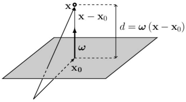 ◄
Let’s write the vector $\mathbf{x}-\mathbf{x}_0$, which starts at the point $\mathbf{x}_0$
(lying on the plane)
and is directed toward the point $\mathbf{x}$ (see the figure on the right; vectors are added according to the triangle rule).
The position of the point $\mathbf{x}_0$ is chosen at the base of the vector $\boldsymbol{\omega}$,
therefore $\boldsymbol{\omega}$ and $\mathbf{x}-\mathbf{x}_0$ are collinear (lie on the same straight line).
If the vector $\boldsymbol{\omega}$ is a unit vector ($\boldsymbol{\omega}^2=1$), then the scalar product of the vectors
$\mathbf{x}-\mathbf{x}_0$ and $\boldsymbol{\omega}$ equals the distance from the point $\mathbf{x}$ to the plane:
$$
d = (\mathbf{x}-\mathbf{x}_0)\cdot \boldsymbol{\omega} ~=~ -\mathbf{x}_0\cdot\boldsymbol{\omega} + \mathbf{x}\cdot\boldsymbol{\omega}
~=~ b + \mathbf{x}\cdot\boldsymbol{\omega}.
$$
◄
Let’s write the vector $\mathbf{x}-\mathbf{x}_0$, which starts at the point $\mathbf{x}_0$
(lying on the plane)
and is directed toward the point $\mathbf{x}$ (see the figure on the right; vectors are added according to the triangle rule).
The position of the point $\mathbf{x}_0$ is chosen at the base of the vector $\boldsymbol{\omega}$,
therefore $\boldsymbol{\omega}$ and $\mathbf{x}-\mathbf{x}_0$ are collinear (lie on the same straight line).
If the vector $\boldsymbol{\omega}$ is a unit vector ($\boldsymbol{\omega}^2=1$), then the scalar product of the vectors
$\mathbf{x}-\mathbf{x}_0$ and $\boldsymbol{\omega}$ equals the distance from the point $\mathbf{x}$ to the plane:
$$
d = (\mathbf{x}-\mathbf{x}_0)\cdot \boldsymbol{\omega} ~=~ -\mathbf{x}_0\cdot\boldsymbol{\omega} + \mathbf{x}\cdot\boldsymbol{\omega}
~=~ b + \mathbf{x}\cdot\boldsymbol{\omega}.
$$
If the length $\omega=|\boldsymbol{\omega}|$ of the normal vector $\boldsymbol{\omega}$ to the hyperplane is not equal to one, then $d$ is $\omega$ times greater ($\omega > 1$) or smaller ($\omega < 1$) than the Euclidean distance in $n$-dimensional space. When the vectors $\mathbf{x}-\mathbf{x}_0$ and $\boldsymbol{\omega}$ are directed oppositely, we have $d < 0$. ►
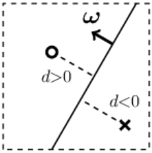 If the space has $n$ dimensions,
then a hyperplane is an $(n-1)$-dimensional object.
If the space has $n$ dimensions,
then a hyperplane is an $(n-1)$-dimensional object.
It divides the entire space into two
parts.
For clarity, let’s consider a 2-dimensional space.
In it, a hyperplane will be a straight line (a one-dimensional object).
In the figure on the right, the circle represents one point in space,
and the cross - another. They are located on opposite sides of the line (the hyperplane).
If the length of the vector $\boldsymbol{\omega}$ is much greater than one, then the distances
$d$
from the points to the plane in absolute value will also be significantly greater than one.
Regression (real number prediction)
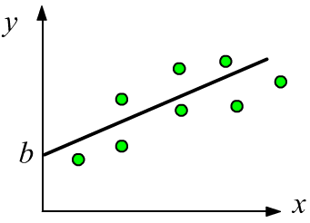 The simplest example of regression is a one-dimensional linear function $y = b + w \,x$,
where the parameter $w$ characterizes the slope of the line, and the parameter $b$ represents the shift (offset) along the $y$-axis from the origin.
Such a relationship between $x$ and $y$ is usually easy to detect visually on a data plot.
The simplest example of regression is a one-dimensional linear function $y = b + w \,x$,
where the parameter $w$ characterizes the slope of the line, and the parameter $b$ represents the shift (offset) along the $y$-axis from the origin.
Such a relationship between $x$ and $y$ is usually easy to detect visually on a data plot.
In the multidimensional case $y=b + w_1x_1+...w_n x_n$, it is more difficult to visualize the data. To verify the adequacy of the linear model, it is necessary to find the optimal parameters and calculate the error value (comparing it with the errors of other models, including the trivial one $y=b=\text{const}$).
Logistic regression (classification problem)
 In a classification problem, an object $\mathbf{x}$ must be assigned to one or more
classes, with the total number $C$ of classes being fixed.
Usually, the result of classification is $C$ conditional probabilities $p(c|\mathbf{x})$ indicating that
an object with features $\mathbf{x}$ belongs to the $c$-th class: $c\in [0...C-1]$.
In a classification problem, an object $\mathbf{x}$ must be assigned to one or more
classes, with the total number $C$ of classes being fixed.
Usually, the result of classification is $C$ conditional probabilities $p(c|\mathbf{x})$ indicating that
an object with features $\mathbf{x}$ belongs to the $c$-th class: $c\in [0...C-1]$.
When using a linear model for a classification problem, its outputs $y_\alpha$ are passed through a nonlinear function $z_\alpha=f(y_\alpha)$, whose values lie in the range $[0...1]$. The closer $z_\alpha$ is to one, the more confidently the model assigns the object to the class with index $\alpha$.
$$ z_{\alpha} ~=~f(\mathbf{y}) ~=~f\Bigr(b_\alpha + \sum_{\mu} x_{\mu}\, w_{\mu \alpha} \Bigr) $$If an object can belong to multiple classes (overlapping classes), then it is convenient to use the sigmoid function as $f(z)$. If the model outputs values close to one on several outputs, then the object belongs to all those classes. For large $y_\alpha$, the sigmoid tends to one, and for $y_\alpha\to -\infty$, it tends to zero: $\sigma(y_\alpha) = 1/(1+e^{-y_\alpha})$
For non-overlapping classes $C > 2$ (the object $\mathbf{x}$ belongs to only one class), the softmax function is typically used. Its outputs are positive values whose sum equals one. Therefore, they can be interpreted as a probability distribution $p(c|\mathbf{x})$: $$ z_\alpha = \mathrm{sm}(y_\alpha) = \displaystyle \frac{e^{y_\alpha}}{\sum_\beta e^{y_\beta}},~~~~~~~~~~~~~~~~~~~~~\sum_\alpha z_\alpha = 1,~~~~~~~~~z_\alpha > 0. $$
If the separating planes for $\{y_0,y_1,y_2\}$ are drawn correctly and the classes are linearly separable, then for a point belonging to class $0$, the output values will tend to $\{1,0,0\}$, for class $1$ - $\{0,1,0\}$, and so on.
Bayes' theorem and softmax
There is a remarkable mathematical fact that provides a “theoretical foundation” for the use of the softmax function. Let the examples of each class $c=[0...,C-1]$ in the feature space $\mathbf{x}$ form “clusters” with normal distributions that have identical variance $\mathbf{D}$ and different means $\bar{\mathbf{x}}_c$. Then the conditional probability $p(c|\mathbf{x})$ of an object with features $\mathbf{x}$ belonging to class $c$ is described by a linear model with a softmax function at the output: $$ P(\mathbf{x} | c) \sim e^{-\frac{1}{2}\,(\mathbf{x}-\bar{\mathbf{x}}_c)\,\mathbf{D}^{-1}(\mathbf{x}-\bar{\mathbf{x}}_c)}~~~~~~~~~~~~~ \Rightarrow~~~~~~~~~~~~~ p(c|\mathbf{x}) = \frac{e^{y_c}}{\sum_\alpha e^{y_\alpha}},~~~~~~~\mathbf{y} = \mathbf{b} + \mathbf{x}\mathbf{w}. $$
Naturally, in real-world problems, the classes in the feature space rarely satisfy the original assumption. However, using neural networks, it is often possible to construct an appropriate nonlinear transformation that produces a new feature space where objects belonging to different classes form linearly separable, compact class clusters. Below is the idea of the proof, which can be skipped.🔥 From the definition of conditional probability, we obtain the Bayes’ theorem: $$ p(c|\mathbf{x}) = \frac{p(c,\mathbf{x})}{p(\mathbf{x})} = \frac{p(c)\,P(\mathbf{x}|c)}{p(\mathbf{x})} = \frac{p(c)\,P(\mathbf{x}|c)}{\sum_\alpha p(\alpha)\,P(\mathbf{x}|\alpha)}, $$ where $p(c)$ is the probability that a randomly chosen object belongs to class $c$. Let's expand the product $(\mathbf{x}-\bar{\mathbf{x}}_c)\,\mathbf{D}^{-1}(\mathbf{x}-\bar{\mathbf{x}}_c)$ under the exponent in $P(\mathbf{x} | c)$. The term $-(1/2)\,\mathbf{x}\,\mathbf{D}^{-1}\mathbf{x}$, which appears both in the numerator and denominator of Bayes’ formula, cancels out. The remaining terms and the factor $p(c)$ can be factorized as follows (the inverse covariance matrix $\mathbf{D}^{-1}$ is symmetric): $$ p(c)\,P(\mathbf{x}|c) \sim e^{b_c + \mathbf{x}\,\mathbf{w}_c},~~~~~~~~~ b_c = -\frac{1}{2}\,\bar{\mathbf{x}}_c\,\mathbf{D}^{-1}\bar{\mathbf{x}}_c + \log\, p(c),~~~~~~~~~~ \mathbf{w}_c = \mathbf{D}^{-1}\bar{\mathbf{x}}_c. $$
Batches and matrix multiplication
Let there be 2 features: $\{x_0,x_1\}$ (model input), which determine three target values: $\{y_0,y_1,y_2\}$ (output). The linear relationship between input and output: $$ \left\{\begin{array}{lcl} y_0 &=& b_0+ x_0 \,w_{00} + x_1\, w_{10} \\ y_1 &=& b_1+ x_0 \,w_{01} + x_1\, w_{11} \\ y_2 &=& b_2+ x_0 \,w_{02} + x_1\, w_{12} \end{array} \right. ~~~~~~~~~~~~~~~~~~~~~~~~~~~~~~~ \mathbf{w} = \overbrace{ \begin{array}{|c|c|c|} \hline w_{00} & w_{01} & w_{02} \\ \hline w_{10} & w_{11} & w_{12} \\ \hline \end{array} }^{\displaystyle n_y} \left. \phantom{ \begin{array}{c} \\ \\ \end{array} } \right\} n_x $$ can be written in tabular form (a dot means multiplication of a row by a column):
$$ \begin{array}{|c|c|} \hline b_{0} & b_{1} & b_{2} \\ \hline \end{array} ~~~+~~~ \begin{array}{|c|c|} \hline x_0 & x_1 \\ \hline \end{array} ~\cdot~ \begin{array}{|c|c|c|} \hline w_{00} & w_{01} & w_{02} \\ \hline w_{10} & w_{11} & w_{12} \\ \hline \end{array} ~~~=~~~ \begin{array}{|c|c|} \hline y_{0} & y_{1} & y_{2} \\ \hline \end{array} $$
In machine learning algorithms, computations are performed not on a single example,
but on a set of them - a batch.
Therefore, we represent $\mathbf{x}$ as a 2D matrix,
placing the examples row by row (the first index, starting from zero, is the sample number, and the second index is the feature number in that sample).
Below are $N=4$ examples, $n_x=2$ features, and $n_y=3$ model outputs:
The index dimensions (the shape attribute in numpy)
of the product matrix $\mathbf{x}\cdot\mathbf{w}$ are:
$$
(N,n_x) . (n_x,n_y) = (N,n_y).
$$
When multiplying matrices:
$(\mathbf{x}\cdot\mathbf{w})_{i\alpha} = \sum_\mu x_{i\mu}\,w_{\mu\alpha}$
the principle "row by column" applies,
and the dimension of the middle index is reduced.
A vector $\mathbf{b}$ of shape (ny,)
is added to each row of the matrix $\mathbf{x}\cdot\mathbf{w}$ of shape (N,ny).
In the numpy library this follows
the broadcasting rule.
Tensor analysis
Next, derivatives with respect to tensors will be computed and matrix notations will be used. Therefore, let's recall some important points.
☝ The matrix inverse of a matrix $\mathbf{A}$ is denoted as $\mathbf{A}^{-1}$, and the transpose as $\mathbf{A}^{\top}$. For a transposed matrix, columns and rows (indices) are swapped: $A^\top_{ij}=A_{ji}$, and the product of the inverse with the original gives the identity matrix (Kronecker symbol). They have the following properties: $$ \mathbf{A}^{-1}\cdot\mathbf{A}=\mathbf{A}\cdot\mathbf{A}^{-1}=\mathbf{1},~~~~~~~~~~ (\mathbf{A}\cdot\mathbf{B})^{-1} = \mathbf{B}^{-1}\cdot\mathbf{A}^{-1},~~~~~~~~~~ (\mathbf{A}\cdot\mathbf{B})^{\top} = \mathbf{B}^{\top}\cdot\mathbf{A}^{\top}. $$
☝ The formula for a partial derivative (the ellipsis are other indices) holds:
$$ \frac{\partial W_{\mu\nu...}}{\partial W_{\alpha\beta...}} = \delta_{\mu\alpha}\,\delta_{\nu\beta}\,...,~~~~~~~~~~~~~~ \sum_{\mu} T_{...\mu...}\,\delta_{\mu\alpha} = T_{...\alpha...}, $$where $\delta_{\alpha\beta}$ is the identity square matrix (Kronecker symbol), equal to $0$ if $\alpha\neq\beta$ and $1$ if $\alpha=\beta$. When summing with the Kronecker symbol (over one of its indices), the sum and the Kronecker symbol are removed, and the summation index is replaced by the second index of the Kronecker symbol (see the second formula above).
The formula for $\partial W_{\mu\nu}/\partial W_{\alpha\beta}$ means that the derivative is zero if $\mu\neq\alpha$ and $\nu\neq\beta$. For example, $\partial W_{12}/\partial W_{13} = 0$ because these are different variables (like $\partial y/\partial x = 0$), while $\partial W_{12}/\partial W_{12} = 1$ (like $\partial x/\partial x = 1$).
Analytical solution
In a linear model with mse error, it is analytically straightforward to find the optimal parameters. The calculations become significantly simpler if the vector $\mathbf{b}$ and the matrix $\mathbf{w}$ are combined into a single matrix $\mathbf{W}$ by adding the vector $\mathbf{b}$ as an additional row to $\mathbf{w}$. Additionally, a column of ones is added to the matrix $\mathbf{x}$, resulting in the matrix $\mathbf{X}$:
$$ \mathbf{X}\cdot\mathbf{W} ~=~ \begin{array}{|c|c|c|} \hline x_{00} & x_{01} & ~1~ \\ \hline x_{10} & x_{11} & 1 \\ \hline x_{20} & x_{21} & 1 \\ \hline x_{30} & x_{31} & 1 \\ \hline \end{array} ~\cdot~ \begin{array}{|c|c|} \hline w_{00} & w_{01} & w_{02} \\ \hline w_{10} & w_{11} & w_{12} \\ \hline b_{0} & b_{1} & b_{2} \\ \hline \end{array} ~=~ \begin{array}{|c|c|c|} \hline y_{00} & y_{01} & y_{02} \\ \hline y_{10} & y_{11} & y_{12} \\ \hline y_{20} & y_{21} & y_{22} \\ \hline y_{30} & y_{31} & y_{32} \\ \hline \end{array} ~=~ \mathbf{y}. $$ This notation introduces an extra dummy feature always equal to one: $\mathbf{x}=\{x_0,...,x_{n-1},1\}$.Now the model takes the form: $\mathbf{y} = \mathbf{X}\cdot\mathbf{W}$, which, as can be easily verified, is equivalent to the original expression $\mathbf{y}=\mathbf{b} + \mathbf{x}\mathbf{w}$. Let's find the minimum of the mse error $L$ (ignoring the constant factor):
$$ L = \sum_{i,\nu} (y_{i\nu} -\hat{y}_{i\nu} )^2,~~~~~~~~~~~~~~~ y_{i\nu} = \sum_{\mu} X_{i\mu} W_{\mu\nu}. $$Let's write down the derivatives of the error and model output: $$ \frac{\partial L}{\partial y_{i\nu}}~=~ 2(y_{i\nu} -\hat{y}_{i\nu} ),~~~~~~~~ \frac{\partial y_{i\nu}}{\partial W_{\alpha\beta}} = \sum_{\mu} X_{i\mu}\,\delta_{\mu\alpha}\,\delta_{\nu\beta}. ~=~X_{i\alpha} \,\delta_{\nu\beta}. $$ Now it is straightforward to compute the derivative of the error $L$ with respect to the elements of the matrix $W_{\alpha\beta}$: $$ \frac{\partial L}{\partial W_{\alpha\beta}} = \sum_{i,\nu} \frac{\partial L}{\partial y_{i\nu}}\,\frac{\partial y_{i\nu}}{\partial W_{\alpha\beta}} ~=~ 2 \sum_{i} (y_{i\beta} -\hat{y}_{i\beta} )\, X_{i\alpha} ~=~2 \bigr[\mathbf{X}^\top\cdot(\mathbf{y}-\hat{\mathbf{y}} )\bigr]_{\alpha\beta}. $$
By setting the derivative to zero (the extremum condition, which in this case corresponds to the minimum of $L$), we obtain the matrix equation $\mathbf{X}^\top\cdot(\mathbf{X}\cdot\mathbf{W}-\hat{\mathbf{y}} ) = 0$, which can be easily solved:
$$ \mathbf{W} = (\mathbf{X}^\top\cdot \mathbf{X})^{-1}\cdot (\mathbf{X}^\top\cdot \hat{\mathbf{y}}) ~~~~~~~~\text{or}~~~~~~~~~~~~~~ \mathbf{W}= \mathbf{X}^{-1} \cdot \hat{\mathbf{y}}. $$In principle, either of these formulas can be used. The first formula is faster if the number of examples N is significantly greater than the number of features nX = number of inputs $\mathbf{x}$. Finding the inverse of the square matrix $\mathbf{X}^\top\cdot \mathbf{X}$ of shape (nX+1, nX+1) is easier than for the matrix $\mathbf{X}^{-1}$ of shape (nX+1, N) in the second formula, although this requires the additional multiplication of matrices $\mathbf{X}^\top\cdot \mathbf{X}$.
Examples using numpy
Let's perform the calculations using the obtained formulas with the numpy library. A brief introduction to numpy can be found in the document NN_Base_Numpy.
First, let's generate model data in which the outputs are linearly related to the inputs with a small random noise added:
import numpy as np                                    # working with tensors

N      = 100                                          # number of points (examples)
nX, nY = 2, 3                                         # number of inputs (features) and outputs

w = np.array([[  1,  3,  5],                          # matrix w of shape (nX,nY)
              [  6,  4,  2] ])
b = np.array( [ -3, -2, -1]  )                        # vector b of shape (nY, )

X  = np.random.random ((N, nX))                       # uniform random points in [0...1]
Y  = np.dot(X, w) + b                                 # model outputs
Y += np.random.normal (0, 0.01, (N, nY))              # add Gaussian noise
Now let's compute the matrices of the linear model using the first and second formulas. Since the matrix in the second formula is not square, to find its inverse we use the pinv function, rather than inv as in the first case:
from numpy.linalg import inv, pinv                    # inverses for square and rectangular matrices

XX = np.concatenate( (X, np.ones((N, 1))), axis=1)    # add a column of ones

W1 = np.dot( inv(np.dot(XX.T, XX)), np.dot(XX.T, Y) ) # first formula
W2 = np.dot( pinv(XX), Y)                             # second formula
Regression using sklearn
To solve the same problem, in practice it is more convenient to use the ready-made machine learning library Scikit-learn (sklearn for short):
from sklearn.linear_model import LinearRegression

lr = LinearRegression().fit(X,Y)

print(lr.coef_.T)                   #  [[1.007  3.001  5.001]  matrix W
                                    #   [6.003  4.     1.998]]
print(lr.intercept_)                #  [-3.002 -2.001 -0.999]  vector b
Calling LinearRegression() creates an instance of the class for this learning method, to which the training data X,Y are passed via the fit function. This function returns the class instance, whose attributes contain the model parameters. Note that the weight matrix $\mathbf{w}$ (attribute lr.coef_) in sklearn is stored in transposed form (compared to the convention used above).
After obtaining the model parameters, its mse error can be computed:
mse =  np.mean((X @ lr.coef_.T + lr.intercept_ - Y) ** 2)

print(f"mse:{mse:.5f}, sqrt(mse):{np.sqrt(mse):.5f} ")
#       mse:0.00010,   sqrt(mse):0.01005
Classification using sklearn
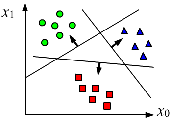
The classification problem with nonlinear sigmoid or softmax functions at the output of a linear model does not have such a simple solution. Therefore, numerical methods must be applied, among which in machine and deep learning the most effective turned out to be gradient descent. Nevertheless, in the linear case it is possible to successfully solve a multiclass classification problem by abandoning the nonlinearity at the model output.
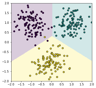
For clarity, consider a two-dimensional feature space $\mathbf{x}=\{x_0, x_1\}$ and three classes $c=\{0,1,2\}$, one of which the object must be assigned to. The model will have three outputs: $n_y=3$, for which we will require the target values for the first, second, and third classes respectively: $$ \mathbf{y}=\{+1,-1,-1\},~~~~~\mathbf{y}=\{-1,+1,-1\},~~~~~\mathbf{y}=\{-1,-1,+1\}. $$ We will still use the mean squared error, for which there is an exact solution. Of course, the linear model will not be able to achieve the target values for all examples. However, the three outputs of the model $\mathbf{y}=\{d_0,d_1,d_2\}$ are three signed distances from the point $\mathbf{x}$ to the three planes. Distances are positive if the normal vector "faces" the point and negative if it points in the opposite direction. The least squares method will try to rotate these vectors so that, at least, the signs of the model outputs match the target values. This will give the required classifier.
Let's prepare model data in the form of three clusters with normally distributed points around their centers:
nx, ny, N = 2, 3, 300                    # number of features, classes, objects (points)

C = np.zeros(N)                          # correct class labels
Y = np.full((N,ny), -1)                  # N x ny output matrix filled with -1
X = np.random.normal (0, 0.4, (N,nx))    # cloud of N points centered at the origin

X0 = [[-1,1], [1,1], [0,-1]]             # centers of clusters for each class
nc = int(N/ny)                           # number of examples per class

for i, x0 in enumerate(X0):
    C[i*nc:(i+1)*nc]    = i              # label of the i-th class
    Y[i*nc:(i+1)*nc, i] = 1              # target outputs
    X[i*nc:(i+1)*nc]   += np.array(x0)   # shift the i-th class cluster
We define the classification model as a class:
class Model:
    def __init__(self):
        "Constructor"
        self.lr = LinearRegression()

    def __call__(self, x):
        "Functional call of the object"
        y = x @ self.lr.coef_.T + self.lr.intercept_
        return np.argmax(y, axis=1)

    def fit(self, x,y):
        "Training on examples x,y"
        self.lr.fit(x,y)
The training and testing process looks like this:
model = Model()       # instantiate model

model.fit(X,Y)        # train

y = model(X)          # get class labels
A = (y==C).mean()     # compare with true labels (accuracy)
To get a plot like at the beginning of the section, add the following method to the Model class:
.   def plot(self, x1_min=0, x1_max=1, x2_min=0, x2_max=1, n=201):
        # 201 x 201 grid of points in the interval x1,x2=[xMin,xMax]
        x1,x2 = np.meshgrid(np.linspace(x1_min, x1_max, n),
                            np.linspace(x2_min, x2_max, n))
        grid  = np.c_[x1.ravel(), x2.ravel()]     # shape = (n*n, 2)

        yp = self(grid).reshape(x1.shape)         # (n*n, ) -> (n, n)

        fig,ax = plt.subplots(figsize=(5, 5))     # figure size (square)
        plt.axis([x1_min,x1_max, x2_min,x2_max])  # axis ranges

        plt.imshow(yp, interpolation='nearest',   # color map for 2D array yp
                  extent=(x1.min(), x1.max(), x2.min(), x2.max()),
                  aspect='auto', origin='lower', alpha=0.2,
                  vmin=0, vmax=yp.max())
With this method, we can plot the decision surfaces and the training points:
model.plot(-2, 2,  -2, 2)
plt.scatter(X[:,0], X[:,1], c=C, s=30, edgecolors='black')
plt.show()
