ML: Gradient Method
Introduction
This document continues the discussion of the multidimensional linear model. Using this model as an example, we will examine the stochastic gradient descent method and the selection of optimal hyperparameters. The Python code using the Numpy, PyTorch and Keras libraries can be found in the file: ML_Line_Model.ipynb.
Gradient method
In complex models, finding an exact analytical expression for the optimal parameters is difficult. Therefore, approximate numerical methods are used, based on the fact that the antigradient of a function locally points in the direction of its decrease.
Let's denote the set of parameters by the vector $\mathbf{w}$. The error is a function of them, $L=L(\mathbf{w})$. In the parameter space, there exist surfaces of constant values $L(\mathbf{w})=\mathrm{const}$. A displacement $d\mathbf{w}$ along such surfaces does not change $L$, and therefore its differential is zero:

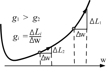
 Thus, the gradient vector $\mathbf{g}$ is perpendicular to the surfaces
$L=\mathrm{const}$ and is directed toward increasing $L$ (as is any derivative).
When approaching a minimum, the gradient length usually decreases, and at the minimum point (an extremum) it becomes zero (see the second figure above).
Thus, the gradient vector $\mathbf{g}$ is perpendicular to the surfaces
$L=\mathrm{const}$ and is directed toward increasing $L$ (as is any derivative).
When approaching a minimum, the gradient length usually decreases, and at the minimum point (an extremum) it becomes zero (see the second figure above).
To find the minimum of $L$, it is necessary to move
in the direction opposite to the gradient (along the antigradient), with a step proportional to some number $\lambda$.
This hyperparameter is called the learning rate:
The larger the learning rate $\lambda$, the faster the model parameters approach their optimal values. However, for large $\lambda$ there is a risk of overshooting the minimum (despite the decrease of the gradient length in its vicinity). We will illustrate this with examples.
✍ In the one-dimensional case, the equation of a parabola with a minimum at the point $w=0$ and its "gradient" $g$ take the form: $$ L(w)=\frac{1}{2}\,\Gamma\,w^2,~~~~~~~~~~~~~g=\frac{dL}{dw}=\Gamma\,w, $$ where $\Gamma$ is a constant. Descent with rate $\lambda$ from the point $w^{(0)}$ brings us, at iteration $t$, to the point: $$w^{(t)}=(1-\lambda\,\Gamma)^t\,w^{(0)}.$$ For $\lambda > 1/\Gamma$, the method becomes unstable: $w^{(t)} \to \pm \infty$. However, the closer $\lambda$ approaches from below the critical value $\lambda_c = 1/\Gamma$, the faster the minimum is reached.
✍
 Gradient descent behaves similarly for "a multidimensional parabola" with different coefficients $\Gamma_i$
for each coordinate:
$$
L = \frac{1}{2}\sum_i \Gamma_i\,w_i ^2,~~~~~~~~~g_i = \Gamma_i\, w_i,~~~~~~w^{(t)}_i=(1-\lambda\Gamma_i)^t\,w^{(0)}_i.
$$
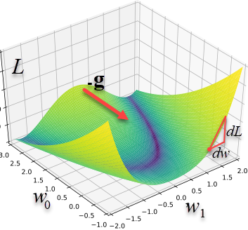
If we are at a point $\mathbf{w}$, the shortest path to the minimum $\mathbf{w}_{\text{min}}=\mathbf{0}$ is in the direction of the vector $-\mathbf{w}$.
However, the gradient method will change the parameters in a different direction, $-\mathbf{g}$,
and will lead to the minimum in "a roundabout way". On the right are shown the trajectories leading to the minimum $\{0,0\}$ in the two-dimensional case
from various initial positions with $\Gamma=\{5, 1\}$ and $\lambda=0.1$.
Note not only the curvature of the trajectories but also the noticeable reduction of the step size as the minimum is approached.
The critical value $\lambda_c$ is determined by the largest coefficient of the parabola: $\lambda_c = 1/\max \Gamma_i = 0.2$.
Gradient descent behaves similarly for "a multidimensional parabola" with different coefficients $\Gamma_i$
for each coordinate:
$$
L = \frac{1}{2}\sum_i \Gamma_i\,w_i ^2,~~~~~~~~~g_i = \Gamma_i\, w_i,~~~~~~w^{(t)}_i=(1-\lambda\Gamma_i)^t\,w^{(0)}_i.
$$
If we are at a point $\mathbf{w}$, the shortest path to the minimum $\mathbf{w}_{\text{min}}=\mathbf{0}$ is in the direction of the vector $-\mathbf{w}$.
However, the gradient method will change the parameters in a different direction, $-\mathbf{g}$,
and will lead to the minimum in "a roundabout way". On the right are shown the trajectories leading to the minimum $\{0,0\}$ in the two-dimensional case
from various initial positions with $\Gamma=\{5, 1\}$ and $\lambda=0.1$.
Note not only the curvature of the trajectories but also the noticeable reduction of the step size as the minimum is approached.
The critical value $\lambda_c$ is determined by the largest coefficient of the parabola: $\lambda_c = 1/\max \Gamma_i = 0.2$.
Stochastic Gradient Descent
SGD (Stochastic Gradient Descent) is a more advanced gradient-based optimization method. Instead of computing the error $L$ over the entire dataset, it evaluates it on a small sample (a batch) of size batch_size. This accelerates convergence because each optimization step requires only a subset of the data rather than the full dataset. After every parameter update, the batch changes, which is why the method is called "stochastic." One full pass over all N examples (one epoch) consists of int(N/batch_size) iterations (steps in parameter space).
Since the amount of data used to compute $\mathbf{g}$ is small (typically batch_size = 10–300), the gradient may fluctuate in different directions from one iteration to the next. To reduce this effect, the gradient vector $\mathbf{g}$ is smoothed into an average value $\langle\mathbf{g}\rangle$ using an exponential moving average. The same smoothing helps traverse a surface with small oscillations. The smoothing strength is controlled by the parameter $\beta=[0...1)$. Starting with $\langle\mathbf{g}\rangle_{(-1)}=0$, the SGD iterations $t=0,1,2,...$ take the form:
$$ \mathbf{w}^{(t+1)} = \mathbf{w}^{(t)} - \lambda \,\langle\mathbf{g}\rangle^{(t)},~~~~~~~~~~~~ \langle\mathbf{g}\rangle^{(t)} = \beta\,\langle\mathbf{g}\rangle^{(t-1)} + (1-\beta)\,\mathbf{g}^{(t)}. $$The parameters batch_size and $\beta$ are correlated. Larger values of either result in stronger smoothing of the gradient. Increasing batch_size reduces training speed (fewer iterations per epoch). However, on GPUs, due to efficient large-matrix multiplications, increasing batch_size can reduce the total training time per epoch, even per iteration.
☝ The moving average of the gradient has the following interpretation. A weighted sum is computed using $\beta$ and $1-\beta$ (whose sum is equal to 1) between the previous average $\langle\mathbf{g}\rangle^{(t-1)}$ and the current gradient $\mathbf{g}^{(t)}$. The closer $\beta$ is to 1, the stronger the smoothing: $\langle\mathbf{g}\rangle^{(t)}\approx \langle\mathbf{g}\rangle^{(t-1)}$. For $\beta=0$, no smoothing occurs and $\langle\mathbf{g}\rangle^{(t)} = \mathbf{g}^{(t)}$.
Below is an illustration of smoothing using a moving average. The blue line represents a one-dimensional stochastic random walk (similar to a stock price). The yellow and green curves show smoothed versions for different values of $\beta$.
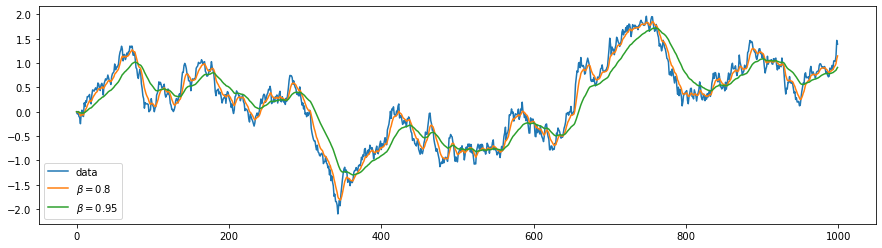
Naturally, the stronger the smoothing (the closer $\beta$ is to 1), the more the averaged curve lags behind the underlying data.
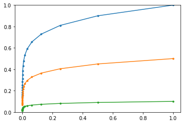
If the averaged value is equal to the constant, $\mathbf{g}^{(t)}=\mathbf{g}=\text{const}$, then after sufficiently many iterations the average converges to the same constant (a geometric series): $\langle\mathbf{g}\rangle^{(1)} = \beta\,\mathbf{0} + (1-\beta)\,\mathbf{g}$, $$ \langle\mathbf{g}\rangle^{(2)} =\beta\,\langle\mathbf{g}\rangle^{(1)}+ (1-\beta)\,\mathbf{g}=(1+\beta)(1-\beta)\mathbf{g},....~~~~~~~~ \langle\mathbf{g}\rangle^{(t)} = (1+\beta+...+\beta^{t-1})(1-\beta)\,\mathbf{g} = (1-\beta^t)\,\mathbf{g}. $$
☝ In the PyTorch and Keras libraries, the parameter $\beta$ is called momentum, and the learning rate lr corresponds to $\lambda\,(1-\beta)$ and $\langle\mathbf{g}\rangle^{(t)} \mapsto (1-\beta)\langle\mathbf{g}\rangle^{(t)}$. In addition, the SGD method "includes support for momentum, learning rate decay, and Nesterov momentum". Learning rate decay refers to reducing lr each epoch (iterations) according to the decay parameter (code from Keras):
lr_t = lr * (1. / (1. + decay * iterations ))Then the following computations occur:
v = momentum * v - lr_t * grad
if nesterov:  params = params + momentum * v - lr_t * grad
       else:  params = params + v
By default, the parameters are: SGD(lr=0.01, momentum=0.0, decay=0.0, nesterov=False).
Gradient computation
Let's compute the gradient of the mean squared error (MSE) for a linear model. We apply the chain rule for differentiating composite functions. In this case, $L$ depends on $y_{i\gamma}$, which themselves depend directly on the parameters: $y_{i\gamma}=\sum_\mu\,x_{i\mu}w_{\mu\gamma}+b_{\gamma}$. Therefore, for the mean squared error $L= \langle (\mathbf{y}-\hat{\mathbf{y}})^2\rangle$, averaged over $N$ samples (first index) and $m$ model outputs (second index), we obtain:
$$ \frac{\partial L}{\partial w_{\alpha\beta}} = \sum_{i, \gamma} \frac{\partial L}{\partial y_{i\gamma}} \, \frac{\partial y_{i\gamma}}{\partial w_{\alpha\beta}} = \frac{2}{N\,m} \sum_{i, \gamma} (y_{i\gamma}-\hat{y}_{i\gamma})\,\sum_\mu\,x_{i\mu}\,\delta_{\mu\alpha}\,\delta_{\gamma\beta} = \frac{2}{N\,m} \sum_{i} x_{i\alpha}\, (y_{i\beta}-\hat{y}_{i\beta}). $$Similarly, for the gradient with respect to $\mathbf{b}$:
$$ \frac{\partial L}{\partial b_{\alpha}} = \frac{2}{N\,m} \sum_{i} (y_{i\alpha}-\hat{y}_{i\alpha}). $$In matrix form, this can be written as:
$$ \frac{\partial L}{\partial \mathbf{w} } = \frac{2}{N\,m}~\mathbf{x}^\top\cdot(\mathbf{y}-\hat{\mathbf{y}}),~~~~~~~~~~~~~ \frac{\partial L}{\partial \mathbf{b} } = \frac{2}{N\,m}~\mathrm{sum}(\mathbf{y}-\hat{\mathbf{y}},~ \mathrm{axis}=0). $$The product $N\,m$ equals the number of elements in the array $\mathbf{y}$, which in numpy is stored in the attribute size.
Numerical search for minimum
The following presents an SGD-based algorithm for searching optimal parameters using the numpy library . The loss is computed on batch_size samples, looping through all training samples for epochs passes:
def Loss(X,Y, W, B):                                     # loss function
    return np.mean((X @ W + B - Y) ** 2)

def My_SGD(X, Y, lr, mo, batch_size, epochs):

    W = np.random.random ((nX, nY))                      # random initial values
    B = np.random.random ((nY, )  )                      # model parameters W,B

    agW, agB, iters = 0, 0, int( len(X)/batch_size )     # averaged gradients, number of batches

    for epoch in range(epochs):                          # an epoch - a full pass through the dataset
        idx = np.random.permutation( len(X) )            # shuffled list of indices
        X, Y = X[idx], Y[idx]                            # shuffle the data

        for i in range(0, iters*batch_size, batch_size): # samples are split into batches
            xb = X[i: i+batch_size]                      # batch inputs
            yb = Y[i: i+batch_size]                      # batch outputs (target values)

            y = xb @ W + B                               # model outputs

            gW = (2 / y.size) * xb.T @ (y - yb)          # gradient with respect to w
            gB = (2 / y.size) * np.sum(y - yb, axis=0)   # gradient with respect to b

            agW = mo*agW + (1-mo)*gW;   W -= lr * agW    # gradients smoothing
            agB = mo*agB + (1-mo)*gB;   B -= lr * agB    # update parameters

    return W, B, Loss(X,Y, W, B)                         # parameters and loss
 Note that the training samples are randomly shuffled
before each epoch.
To achieve this, a shuffled list of integers from 0 to len(X)-1
is created using np.random.permutation.
The next line performs the actual reordering of the data.
Shuffling before each epoch is not strictly required, but when the dataset is small, it can improve convergence to the minimum.
Moreover, if the number of samples N is not divisible by batch_size,
not all data will be included in the gradient calculation. Shuffling mitigates this issue.
Note that the training samples are randomly shuffled
before each epoch.
To achieve this, a shuffled list of integers from 0 to len(X)-1
is created using np.random.permutation.
The next line performs the actual reordering of the data.
Shuffling before each epoch is not strictly required, but when the dataset is small, it can improve convergence to the minimum.
Moreover, if the number of samples N is not divisible by batch_size,
not all data will be included in the gradient calculation. Shuffling mitigates this issue.
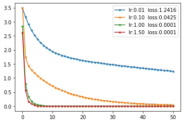
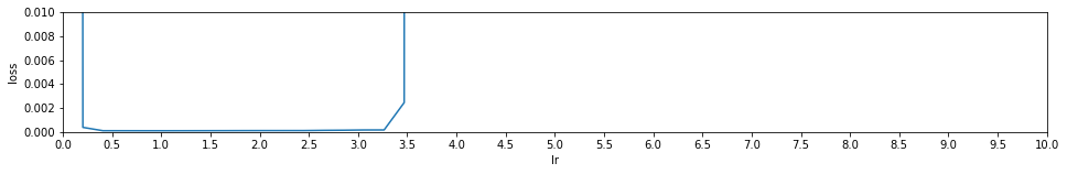
The plots on the right show the loss curves at different learning rates and mo=0. The critical learning rate lr is approximately 1.75. As the value approaches this threshold, the learning rate increases significantly.
Optimal hyperparameters
Any optimization method depends on hyperparameters, and selecting them can sometimes be critically important.
Let's plot an error height map of Loss for a linear model as a function of the
hyperparameters $\lambda$ (=lr) and $\beta$ (=mo).
Blue indicates minimum error, brown indicates maximum.
The number of epochs = 10 and batch_size = 10 are fixed (with N=100 samples).
The light blue line with markers shows the value of $\beta$ corresponding to the minimum error for each $\lambda$.
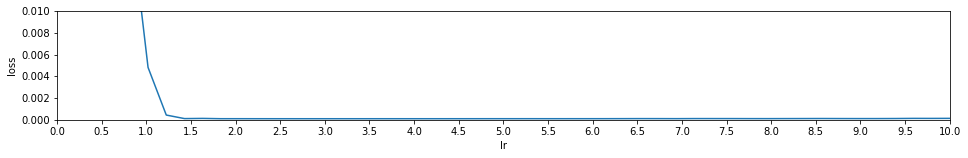
Below the height map is a plot of error as a function of $\lambda$ (using the optimal $\beta$ for each $\lambda$).
Brown regions on the height map correspond to instability of the gradient method:
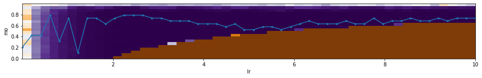
As can be seen, for such a simple model, when $\beta \sim 0.8$, the value of $\lambda$
can vary within a wide range.
The optimal hyperparameters are: mo=0.63, lr=5.31, loss=0.00013.
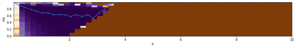
Note that an appropriate parametrization of hyperparameters is important.
For example, if we choose, as in Keras
lr=$\lambda\,(1-\beta)$, the resulting landscape becomes less stable:
Gradient on a Graph in PyTorch
The PyTorch library from Facebook is a popular tool for developing complex neural network architectures. PyTorch creates a dynamic computational graph (it is built during computation and does not require compilation).
Let's reproduce a simple gradient method using PyTorch. The model parameters W,B are terminal nodes of the computational graph, for which the gradient will be computed (requires_grad=True):
The randn method returns a tensor of normally distributed random numbers. By default, they have type float32. To make it match the type of the training data X,Y, the type is explicitly specified using the dtype argument.
Then the main computation loop follows:
import torch

def grad_tourch(X, Y, lr=1, batch_size=10, epochs=10):
    W = torch.randn(nX, nY, dtype=torch.float64,  requires_grad=True)
    B = torch.randn(nY,     dtype=torch.float64,  requires_grad=True)

    for epoch in range(epochs):                          # an epoch - pass through all samples

        idx = torch.randperm( len(X) )                   # shuffled list of indices
        X, Y = X[idx], Y[idx]                            # shuffle the data

        sumL, iters = 0, int( len(X)/batch_size)         # total loss and number of batches

        for i in range(0, iters*batch_size, batch_size): # samples are split into batches

            xb = torch.from_numpy(X[i: i+batch_size])
            yb = torch.from_numpy(Y[i: i+batch_size])

            y = xb.mm(W).add(B)                          # model y = bx @ W + B
            loss = ((y-yb)**2).mean()                    # mse loss for the batch
            sumL += loss.data.item()

            loss.backward()                              # compute gradients

            with torch.no_grad():
                W.add_(- lr *  W.grad)                   # without rebuilding the graph
                B.add_(- lr *  B.grad)

            W.grad.zero_()                               # reset gradients
            B.grad.zero_()

        print(f"{epoch:3d}({iters})  loss:{sumL/iters:0.5f}")

    return W, B

grad_tourch(X, Y)
First, torch tensors for the batches are created from numpy tensors (no new memory is allocated). Then the computational graph is built, whose root is the model loss. At the same time, computations are performed on the graph. Then the backward method is called on the root, which traverses the branches backward and computes gradients.
Any expression involving tensors that have the property requires_grad=True leads to a dynamic reconstruction of the computational graph, leading to its root (the model loss). To prevent this, after backward the no_grad() context is set, which blocks modification of the graph. At the same time, when changing parameters, we do not create new tensors (the add_ function performs in-place "increment"). After changing W,B, it is necessary to reset the gradients to zero (for the next iteration).
Neural network in PyTorch
The parameters of a linear model can also be found using a neural network with a single layer and no activation function:
import torch.nn as nn

model = nn.Sequential( nn.Linear(nX, nY) )
Let's create an SGD optimizer (which will update the parameters) and an mse loss function:
optimizer = torch.optim.SGD(model.parameters(), lr=1, momentum=0.9)
criterion = nn.MSELoss()
The training loop looks as follows. At each iteration, a batch of samples is fed into the network y = model(xb), resulting in a forward pass. The obtained network output y, together with the "true" values yb, is passed to the loss function. For it, backpropagation (backward) is called, as a result of which the gradients are computed. The optimizer's step method updates the model parameters using these gradients. Then the optimizer resets the gradients (zero_grad):
iters = int( len(X)/batch_size )
for epoch in range(epochs):                           # an epoch - pass through all samples
    for i in range(0, iters*batch_size, batch_size):  # samples are split into batches
        bx = torch.Tensor( X[i: i+batch_size] )       # create torch tensors
        by = torch.Tensor( Y[i: i+batch_size] )       # from numpy arrays (float32)

        y = model(bx)                                 # forward pass

        loss = criterion(y, by)                       # compute loss
        loss.backward()                               # compute gradients

        optimizer.step()                              # update parameters
        optimizer.zero_grad()                         # reset gradients

    print('epoch: %d  Loss: %.6f'  % (epoch,  loss) )
After training, the model parameters can be printed:
print(model[0].weight, model[0].bias)The weight matrix, as in sklearn, is stored in transposed form.
Neural network in Keras
The Keras library is an easy-to-use tool for
designing neural networks. Currently, it is an integral part of the tensorflow framework
by Google.
An introduction to Keras can be found in the document NN_Base_Keras.
A linear model (a single layer without an activation function) in Keras is implemented as a fully connected Dense layer. Creating a neural network with one such layer is done as follows:
from   tensorflow       import keras              # keras from tensorflow
from   keras.models     import Sequential         # method for forming layers (stack)
from   keras.layers     import Dense              # fully connected layer
from   keras.optimizers import SGD                # optimization method

model = Sequential()                              # linear stack of layers
model.add(Dense(units=nY, input_dim=nX))
After the model is created, it is compiled and its training (fitting) is started. During training, we will use the SGD optimizer and the mse loss:
model.compile(optimizer = SGD(lr=2, momentum=0.5), loss = 'mse')

res = model.fit(X, Y, batch_size=batch_size, epochs=10,  verbose=0 ) )
After training, one can plot the loss curve as a function of the number of epochs:
plt.plot(res.history['loss'], marker=".")
plt.legend(["loss: %.5f"  % ( res.history['loss'][-1] )])
plt.show()
The parameters of each layer (in our case there is only one layer) are stored in a list returned by the layer method get_weights(). Therefore, the weights and biases of a linear model (or, in the general case, a multilayer fully connected model) are printed as follows:
for lr in model.layers:                           # over all layers
    w = lr.get_weights()[0]                       # synaptic weights of neurons
    b = lr.get_weights()[1]                       # neuron biases
    ...
