ML: Tensors in Keras
Introduction
A neural network is a function $\mathbf{T}' = F(\mathbf{T})$, which transforms one tensor $\mathbf{T}$ into another $\mathbf{T'}$.
There are several frameworks (tensorflow, pytourch), that provide efficient computation of such functions, including on GPU. Initially, the syntax of such frameworks was quite cumbersome, therefore François Chollet wrote a library in the form of keras, which significantly simplified the design of neural networks. Over time keras was absorbed by Google and is now developed only as part of tensorflow version 2.0 and above.
In fact, frameworks not only compute the function $F(\mathbf{T})$ (forward propagation), but also solve a complex optimization problem by adjusting the parameters of the function (backpropagation). Nevertheless, in this document we will focus on the first task. Understanding how the computation of $F(\mathbf{T})$ occurs at each stage is necessary for understanding the operation of complex neural network architectures.
The layers used below will be imported from tensorflow:
from tensorflow.keras.layers  import Input,   Dense, SimpleRNN, Lambda
from tensorflow.keras.layers  import Flatten, Dot,   Activation
Tensors in the backend
The keras library at a low level used to be able to work with numpy, tensorflow, or theano tensors. Therefore, by tradition, it wraps tensors in its own class. For this, the backend environment is used:
import tensorflow.keras.backend as K
Since tensors participate in optimization algorithms, there is a need to distinguish constant and variable tensors:
cnst = K.constant(value = np.array([ [1, 2], [3, 4]]),  # numpy array
                  dtype = 'float32',                    # type of its elements
                  name  = 'my_cnst')                    # name (for references)

print( type ( cnst  ) )     #>  tensorflow.python.framework.ops.EagerTensor
print( cnst )               #>  tf.Tensor( [[1. 2.] [3. 4.]], shape=(2, 2), dtype=float32)
Since keras (outside tensorflow) can work with different backends, the object returned by the method may be either a numpy tensor or a tensorflow tensor. Therefore, their properties should be accessed through backend functions:
print( K.dtype(cnst) )      #>  float32
print( K.int_shape(cnst) )  #>  (2, 2)
Similarly for variables:
var = K.variable(value = np.array([ [1, 2], [3, 4]]),  # numpy array
                 dtype = 'float64',                    # type of its elements
                 name  = 'my_var')                     # name (for references)

print( type ( var  ) )    #>  tensorflow.python.ops.resource_variable_ops.ResourceVariable
print( var )              #>  tf.Variable 'my_var:0' shape=(2, 2) dtype=float64,
                          #>  numpy= array([[1., 2.], [3., 4.]])
Keras tensors can be manipulated similarly to numpy tensors:
t = K.ones((2, 3))                   # 2x3 matrix of ones

t1 = t[:, 0]                         # the first column
t2 = t[:, 1]                         # the second column
t3 = K.concatenate([t1, t2])         # their concatenation into a single vector

print(t1)                            #> tf.Tensor([1. 1.], shape=(2,), dtype=float32)
print(K.eval(t1))                    #> [1. 1.]
print(K.eval(t3))                    #> [1. 1. 1. 1.]

type(t1)                             #> tensorflow.python.framework.ops.EagerTensor
Layer objects
Neural networks consist of interconnected layers Layers are “elementary” functions that form the final model $F(\mathbf{T})$. Each layer is a class. An instance of this class receives a tensor as input and outputs a tensor, generally of a different dimension and shape. Keras layers have two key features:
- When processing a tensor, its zero axis is not affected.
- Declaring a layer does not yet lead to computation.
The first feature is related to the fact that computations are performed not for a single tensor, but for a set of them (batch) of size batch_size. In machine learning tasks, each tensor in a batch is one example. When optimizing model parameters, the error is computed over all examples in the batch.
In fact any Layer is an elementary function that performs computations independently for each example (although it often does this “simultaneously” and very efficiently for all examples at once):
   for i in range(x.shape[0]):
      y[i] = Layer(x[i])
(in numpy, the notation x[i] for a tensor, for example of rank three,
means x[i,:,:] - the i-th matrix of the batch).
The second feature is related to the fact that all tensor transformations form a computational graph. A forward pass through this graph results in computing the tensors (and the neural network output), and a backward pass results in computing the gradients required when optimizing the model parameters.
Activation layer
Let's consider the Activation layer, which computes a specified function for each element of the tensor. The layer has no trainable parameters, and the shape of the output tensor matches the shape of the input.
Let's compute in numpy, for example, the hyperbolic tangent of a tensor of shape (2,3):
val = np.array([ [1, 0, -1],   # val.shape = (2,3)
                 [2, 0, -2]])
y = np.tanh(val)
In the keras library we must convert the input numpy tensor val into a keras tensor x. Then we create an instance "a" of the Activation layer class and pass the input tensor x to it. The layer returns the output tensor y:
x =  K.variable( val )         # keras tensor from numpy tensor val

a = Activation('tanh')         # instance of the Activation object
y = a(x)                       # y - tensor after processing tensor x

print( y )                     # Tensor("activation_10/Tanh:0", shape=(2,3), dtype=float32)

print( K.eval(y) )             # [[ 0.762  0.    -0.762]
                               #  [ 0.964  0.    -0.964]]
Note that the numbers (the actual computations) appear only after calling K.eval(y).
This function starts the execution of the computational graph leading to the node y.
Creating a layer and obtaining the output tensor can be combined in one line. For example, let us compute the softmax function:
y = Activation('softmax')(x)

print(K.eval(y))               # [[0.665 0.245 0.09 ]
                               #  [0.867 0.117 0.016]]
This function $e^{x_{i \alpha}}/\sum_\beta e^{x_{i\beta}}$ uses not only the given element $x_{i\alpha}$,
but also (for normalization) all other elements along the first axis (second index).
As a result, the sum of the numbers for each batch example turns out to be 1
(which is usually used in the final layer to obtain “probabilities” of classes).
Flatten layer
The Flatten layer also has no trainable parameters, but it changes the shape of the tensor.
The task of this layer is to transform a multidimensional input tensor into a one-dimensional tensor (excluding the batch axis!).
In numpy this might look like this:
x = np.arange(12)
x.shape = (2,2,3)              #  input - a stack of two 2x3 matrices

y = x.reshape(x.shape[0], -1)  #  output - a "stack" of vectors

print(y)                       #  [[ 0  1  2  3  4  5]
                               #   [ 6  7  8  9 10 11]]
In keras these same computations look as follows:
x = K.arange(12)               # keras tensor [0,...,11]
x = K.reshape(x, (2,2,3))      # change its shape

f = Flatten()                  # instance of Flatten object
y = f(x)                       # y - tensor after processing tensor x

print( x.shape )               #> (2, 2, 3)
print( y.shape )               #> (2, 6)

print( K.eval(y) )             #> [[ 0  1  2  3  4  5]      <- regular numpy array
                               #   [ 6  7  8  9 10 11] ]
(batch_size, d1,d2,...,dn) => (batch_size, d1*d2*...*dn)
Fully connected Dense layer
The Dense layer consists of units neurons, connected by synapses to the elements of the input tensor along its last index. Let the dimension of this index be inputs = x.shape[-1]. The trainable parameters of the Dense layer are the matrix $\mathbf{W}$ of shape (inputs, units) and the vector $\mathbf{b}$ of shape (units, ). The layer performs a linear transformation:
$$ y_{...j} = \sum^{\mathrm{inputs}-1}_{i=0} x_{...i}\, W_{ij} + b_j, $$where the ellipsis denotes, generally speaking, an arbitrary number of indices besides the mandatory zero batch index: (batch_size,...,inputs) (inputs, units) + (units, ).
Below, as the matrix $\mathbf{W}$, we specify a matrix consisting of ones (if not done, its elements will be random). Using the use_bias parameter, we indicate that we do not need the vector $\mathbf{b}$:
x = K.reshape(K.arange(6, dtype="float32"), (2,3))

W = np.ones((3,4))

d = Dense(units=4, weights = [W], use_bias = False)
y = d(x)

K.eval(y)         # compute the product
In tabular form, the input matrix $\mathbf{x}$ consists of two rows (batch_size=2) and three columns (three features for each of the two samples). Since the number of neurons is units=4, the weight matrix has shape (3, 4):
$$ \mathbf{x}\cdot \mathbf{W} ~=~ _\text{batch_size} \Bigg\{ \overbrace{ \begin{array}{|c|c|c|} \hline 0 & 1 & 2 \\ \hline 3 & 4 & 5 \\ \hline \end{array} }^{\mathrm{inputs}} ~~~\cdot~~~ _\text{inputs} \Bigg\{ \overbrace{ \begin{array}{|c|c|c|c|} \hline 1 & 1 & 1 & 1 \\ \hline 1 & 1 & 1 & 1\\ \hline 1 & 1 & 1 & 1\\ \hline \end{array} }^{\mathrm{units}} ~ = ~ _\text{batch_size} \Bigg\{ \overbrace{ \begin{array}{|c|c|c|c|} \hline 3 & 3 & 3 & 3 \\ \hline 12 & 12 & 12 & 12 \\ \hline \end{array} }^{\mathrm{units}} ~ = ~ \mathbf{y}. $$When adding the bias vector to the matrix, the broadcasting rule is used. According to this rule, the vector is expanded into a matrix (inputs, units) with identical rows.
Note that the dimension of the input tensor can be arbitrary:
x = K.ones((2,3,4,5))
y = Dense(8)(x)

print(y.shape)             # (2, 3, 4, 8)
The matrix inside the Dense layer object is created when an input tensor is attached to it (and the dimension of its last index becomes known):
d = Dense(1)
print( d.weights )   #> []

x = K.ones((2,3))
y = d(x)

print(d.weights)     #> [[-1.132], [ 0.808],  [-0.135]]
(batch_size, d1,d2,...,dn, inputs) => (batch_size, d1,d2,...,dn, units)
Conv2D convolution layer
The convolutional layer Conv2D is applied to “images” with height rows, width cols, and having channels color channels. In fact, these graphical terms are conventional, and the Conv2D layer can be used not only for image processing. It is important that the input tensor must have the shape:
x.shape = (batch_size, channels, rows, cols) if data_format = "channels_first"
x.shape = (batch_size, rows, cols, channels) if data_format = "channels_last" (default)
For clarity, we will use the second order, which is the default in keras.
The task of the Conv2D layer is to process the “image” with a small filter that slides over it. Filtering is performed simultaneously across all channels. In the figure below, the image (input x) has 3 rows, 4 columns, and 2 channels. The kernel size of the filter is 2x2 pixels and 2 in depth for the channels (3D tensor: the blue cube).

The kernel elements (which define the filter) are multiplied by the corresponding elements of the same cube on the image (yellow color). These products are summed and a bias (another filter parameter) is added. The result of the computation is placed into the first pixel of the output y of the layer (blue color). Then the yellow “cube” shifts to the right (by default one pixel) and the next output value is computed.
The layer may have not one but several filters with different kernels and biases (below the blue and light-green cubes). In this case, the computations described above are performed independently for each filter f. The output of the layer will have the number of channels (depth) equal to the number of filters:

The Conv2D layer has two required parameters:
- filters - the number of filters;
- kernel_size = (k_rows, k_cols) - the filter dimensions.
y[s, r, c, f] = np.sum( x[s, r:r+h, r:c+w, :] * ker[:, :, :, f] ) + bias[f].
Convolution in numpy and keras
Let's consider an example of computing a convolution using numpy. Suppose the image has 3 rows, 4 columns, and contains one channel. We fill its left half with ones (“white”) and the right half with zeros (“black”):
channels, filters = 1, 1                          # one channel, one filter
x_rows, x_cols    = 3, 4                          # input image size

im = np.ones((x_rows, x_cols), dtype = 'float32') # left half of the image - "white"
im[:, 2:] = 0                                     # and the right half - "black"
We will process the image with a convolutional layer with one filter and a kernel size of 2x2 (below it will be a vertical edge detection filter). Assume the filter has no bias:
k_rows, k_cols    = 2, 2                          # kernel size

y_rows = x_rows-k_rows+1                          # output image size
y_cols = x_cols-k_cols+1                          # (filter moves one pixel at a time)

x = im.reshape( (1, x_rows, x_cols, channels) )   # input
y = np.empty  ( (1, y_rows, y_cols, filters ) )   # output

ker = np.array( [ 1,-1,  1,-1   ] )               # filter kernel
ker.shape = (k_rows, k_cols, channels, filters)   # vertical edge detection

for r in range(y_rows):                           # convolution
    for c in range(y_cols):
        y[0,r,c,0] = np.sum( x[0, r:r+k_rows, c:c+k_cols, :] * ker[ :, :, :, 0] )
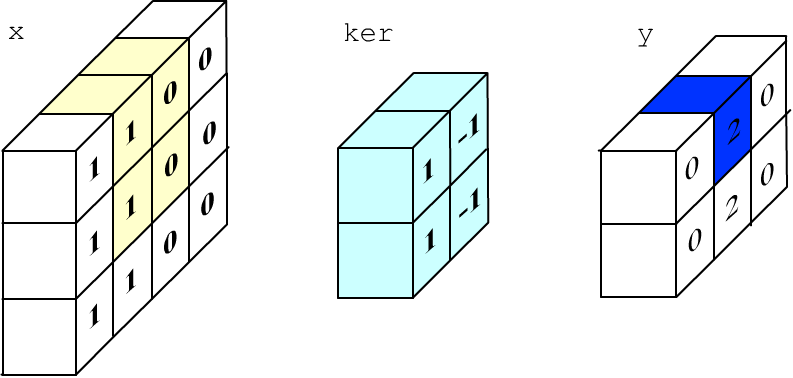
The process of computing a single output pixel is shown in the figure below (1*1+0*(-1)+1*1+0*(-1)=2):
Now let's perform the same computations in keras:
x = K.variable(value = im.reshape( (1, x_rows, x_cols, channels) ))

con = Conv2D(filters = 1, kernel_size = (k_rows, k_cols),
             use_bias = False, weights = [ker] )

print(x.shape,"=>", y.shape)                     #> (1, 3, 4, 1) => (1, 2, 3, 1)
print(K.eval(y).reshape(-1))                     #> [0, 2, 0,
                                                 #   0, 2, 0]
(batch_size, x_rows, x_cols, channels) => (batch_size, y_rows, y_cols, filters)
The values (y_rows, y_cols) depend on (x_rows, x_cols), the filter kernel size (k_rows, k_cols), and how the filter moves over the input image. This movement is determined by the parameters:
- padding - whether to pad the image with zeros so that the number of rows and columns in the output equals the input. If so, padding = "same", otherwise "valid" - then the size is smaller (default).
- stride=1 - how many pixels the filter shifts. In this case (if padding is not used), the output layer has y_rows = (x_rows - k_rows)/stride + 1 and similarly for y_cols.
Universal Lambda layer
If standard-behavior layers do not fit, you can use the Lambda layer. This layer receives an arbitrary lambda function that modifies the input tensor. The only restriction: inside the lambda function, you can only use tensor operations from the backend. Otherwise, keras will not be able to compute the gradient during backpropagation.
For example, let's compute the sum of the components of the input tensor along axis=1 (the second "feature" index):
x = K.variable(value = np.array([[1,2,3],  [4,5,6]]) )

lm = Lambda(lambda t: K.sum(t,axis=1))
y  = lm(x)

print( K.eval(y) )                    #>  [ 6. 15.]
Multiple tensors can be passed to a layer using a list. As a simple example, let's add two tensors inside the lambda function:
x1 = K.variable(value = np.array([[1,2,3],  [4,5,6]]) )
x2 = K.variable(value = np.array([[7,8,9],  [1,2,3]]) )

lm = Lambda(lambda lst: lst[0]+lst[1])
y  = lm([x1,x2])

print( K.eval(y) )                    #> [[ 8. 10. 12.]
                                      #   [ 5.  7.  9.]]
