ML: Word Embedding
Embedding layer
Embedding layer based on contextual frequencies and PCA dimensionality reduction are difficult to use when the vocabulary contains several hundred thousand words. In addition, they do not allow improving the vectorization quality by increasing the complexity of the model. As usual, neural networks come to the rescue.
Neural network frameworks include a special layer called Embedding. This layer receives word indices as input and outputs their vector representations (which are random before training begins):
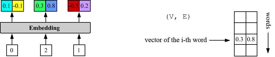
Above, E = 2 and the layer has three inputs (nX = 3). The first word has index 0, the second 2, and the third 1. The Embedding layer stores a matrix of shape (V, E). When the number i is fed into the input, the layer outputs the i-th row of this matrix.
Vector representations (= embedding = Word2Vec) of vocabulary words can be obtained in different ways. For example, the matrix of the Embedding layer can be trained directly on a specific task. Alternatively, you can first obtain "rough" values of vector components using a simplified model and then fine-tune them on a more complex task. Usually, the terms vectorization (or embedding) are used in a general sense. The term Word2Vec is more specific and most often refers to the methods described below: Skip-gram and CBOW.
Skip-gram and CBOW
Suppose we have a long sequence of words (for example, from a natural language): $w_0,w_1,...$. Words that are close in meaning should appear in similar contexts, and the vectors of such words should be close to each other.
In Skip-gram, the training data consist of pairs: a given word $w_t$ and one word from its context. To form such ordered pairs, $(n=2m+1)$-grams are created, where $m$ is the number of words before and after $w_t$: $$ \{w_{t-m},...,w_{t-1},\,\underline{w_{t}}\,,w_{t+1},...,w_{t+m}\} ~~~~~~\Rightarrow~~~~~~ \{~ (w_t, w_{t\pm i}),~~~~~i=1...m~\}. $$
This method exists in two variants. In the Skip-gram Softmax version, one of the context words $w_{t\pm i}$ is predicted from the word $\mathbf{X} = w_t$. At the output of the network, a V-neuron softmax layer is used, which produces the "conditional probabilities": $\mathbf{Y} ~=~ p(w_i| w_t),~~~i=0...V-1$ for all words in the vocabulary. The function $\text{argmax}_{i}\,p(w_i|w_t)$ returns the index $i$ of the most probable word.
In Skip-gram Negative Sampling, both words of the pair $\mathbf{X}=(w_t, w_{t\pm i})$ are fed into the input and belong to the positive class ($Y=1$). Pairs $X=(w_t, w')$, where $w'$ is a random word from the text, belong to the negative class ($Y=0$). If the vocabulary is large enough, the random word $w'$ will most likely not belong to the context of $w_t$. Selecting the random word from the text rather than from the vocabulary preserves its natural frequency distribution. The output of the network is a single neuron with a sigmoid function = [0...1] (binary classification).
CBOW (Continuous Bag of Words) is an alternative Word2Vec method in which the "probability" of the word $w_t$, is predicted from the vectors of all surrounding words (a softmax function with output size V is used): $$ \mathbf{X} = [w_{t-m},...,w_{t-1},w_{t+1},...,w_{t+m}],~~~~~~~~~~Y = w_{t}. $$
Below we consider examples of architectures for these methods. It is believed that Skip-gram works better for rare words (since they are not "hidden" by averaging as in SBOW). However, SBOW uses the context more effectively for predicting the target word.
As with the probabilistic method discussed earlier, these methods group together semantically similar concepts. Consider, for example, the names of the days of the week ("Monday", "Tuesday",..., "Sunday"). They rarely appear next to each other in the same sentence, but they occur in similar contexts: "on Monday morning", "every Monday", "It was a Monday", "one Monday", where any day of the week could replace Monday. As a result, all days of the week, rotating their vectors toward the vectors of context words, tend to move toward a common region of the vector space, where the "combined force" from context words pulls them.
Word pairs for the Skip-gram method
Pairs for the Skip-gram method are constructed from words that fall within a symmetric window WIN around the central word in the list words inside a sentence:
def get_pairs(words, WIN, pairs):
    for i1, w1 in enumerate(words):
        if not w1 in word_to_id: continue

        i2_beg = max(0, i1-WIN)
        for i2 in range(i2_beg, min(len(words), i1+WIN+1) ):  # around  w1
            if i2 != i1 and words[i2] in word_to_id:
               pairs.append((w1, words[i2]))
For example, after the sentence
"['the', 'cat', 'likes', 'the', 'mat']"
with the window WIN=2, we obtain the following set of pairs:
('the',   'cat'), ('the',   'likes'),
('cat',   'the'), ('cat',   'likes'), ('cat',   'the'),
('likes', 'the'), ('likes', 'cat'),   ('likes', 'the'), ('likes', 'mat'), ...
Since the sentences in the corpus we use are relatively short, we choose a large window WIN, assuming that all words in a sentence form the context for any word in that sentence:
pairs = []                                     # list of pairs
for doc in docs:                               # iterate over documents
    for sent in doc:                           # iterate over document sentences
        get_pairs(sent.split(), 100,  pairs)
Before constructing training samples, it is advisable to shuffle the pairs:
import random
random.shuffle(pairs)                          # shuffle randomly
In the ROCStories corpus (see file 100KStories.zip), when constructing pairs within a sentence with WIN = 100, we obtain 45'671'880 pairs (with a vocabulary of 10'393 words).
Skip-gram Softmax
In the pair $(\mathbf{u},\mathbf{w}_i)$ the vector of the "central" word $\mathbf{u}$ and the vector of the context word $\mathbf{w}_i$ are considered to belong to different embeddings (i.e., we distinguish the central word from the words in its context). This means that $\mathbf{u}$ and $\mathbf{w}$ are rows of different matrices of the same shape (V, E). The degree of similarity between words is characterized by the dot product of vectors $\mathbf{u}\mathbf{w}_i$ (parallel vectors correspond to semantically close words). Given the vector of the central word $\mathbf{u}$ as the input of the model, the output predicts the probability distribution of its context words. For this purpose, the softmax function is used (the denominator sums over all vocabulary words $\mathbf{w}_j$): $$ p_i = \frac{e^{\mathbf{u}\mathbf{w}_i}}{\sum_j e^{\mathbf{u}\mathbf{w}_j}}. $$ If the pair consists of words with indices (i,j), then the model input $\mathbf{X}$ will receive the integer i (the word index), and at the output $\mathbf{Y}$ we expect a vector p=[0,0,...,0,1,0,..,0], where the 1 is at position j. To save memory, only the index j is stored for the output $Y$ (sparse encoding for CrossEntropyLoss in PyTorch):
X = np.zeros((len(pairs), 1),   dtype=np.int64)
Y = np.zeros((len(pairs)),      dtype=np.int64)

for i, (u,w) in enumerate(pairs):
    X[i,0] = wordID[u]["id"]          # index of input (central) word
    Y[i]   = wordID[w]["id"]          # index of predicted word
The simplest implementation of the Skip-gram method in PyTorch is:
E_DIM   =  100                                               # vector dimension

model = nn.Sequential(                                       # (N,1)   input X
        nn.Embedding(V_DIM, E_DIM, scale_grad_by_freq=True), # (N,1,E)
        nn.Flatten(),                                        # (N,E)
        nn.Linear   (E_DIM, V_DIM, bias=False))              # (N,V)   CrossEntropyLoss
The Embedding layer stores the vectors of the "central" words
and has V*E parameters.
The input $\mathbf{X}$ has shape (N,1), where N
is the number of samples in the batch.
After the Embedding layer we obtain the tensor $\mathbf{X}_e:$ (N,1,E).
The Flatten layer changes its shape to $\mathbf{X}_f:$ (N,E).
The parameter scale_grad_by_freq specifies that during training,
vectors of rare words in the batch should be updated more strongly than those of frequent words.
Naturally, the batch size should therefore be increased (for example N=512).
The fully connected Linear layer (without bias) contains a weight matrix $\mathbf{W}$ of shape (V, E) with the same number of parameters as in the Embedding layer. This matrix represents the list of vectors $\mathbf{w}_i$. In the linear layer the multiplication $\mathbf{X}_f\cdot\mathbf{W}^\top$ is performed, where $\mathbf{W}^\top$ is the transposed matrix. Since each row of the training data contains the vector of the input word $\mathbf{u}$, it is multiplied with all vectors $\mathbf{w}_i$, and after passing through softmax we obtain probabilities $p_i$. In PyTorch, the softmax function is computed inside the loss CrossEntropyLoss, so it does not need to be explicitly included in the network output.
$$ \text{N} \left\{ \phantom{ \begin{array}{} \\ \\ \\ \\ \end{array} } \right. \overbrace{ \underbrace{ \begin{array}{|c|c|c|} \hline u_1 & u_2 & u_3 \\ \hline ~ & ~ & ~ \\ \hline ~ & ~ & ~ \\ \hline ~ & ~ & ~ \\ \hline \end{array} }_ {\mathbf{u}} }^ {\displaystyle\mathrm{E}} ~~~ \cdot ~~~ \text{E}\left\{ \phantom{ \begin{array}{} \\ \\ \\ \end{array} } \right. \overbrace{ \underbrace{ \begin{array}{|c|c|c|c|c|} \hline ~ & ~ & w_{i1} & ~ & ~ \\ \hline ~ & ~ & w_{i2} & ~ & ~ \\ \hline ~ & ~ & w_{i3} & ~ & ~ \\ \hline \end{array} }_ {\mathbf{W}^\top} }^ {\displaystyle\mathrm{V}} ~~~~~~=~~~~~~ \text{N} \left\{ \phantom{ \begin{array}{} \\ \\ \\ \\ \end{array} } \right. \overbrace{ \underbrace{ \begin{array}{|c|c|c|c|c|} \hline ~ & ~ & \mathbf{u}\mathbf{w}_i & ~ & ~\\ \hline ~ & ~ & ~ & ~ & ~\\ \hline ~ & ~ & ~ & ~ & ~\\ \hline ~ & ~ & ~ & ~ & ~\\ \hline \end{array} }_{\mathrm{softmax}~~ \Rightarrow~~ p_i} }^ {\displaystyle\mathrm{V}} $$The matrix of vectors is stored in model[0].weight, and the output layer matrix in model[2].weight. After training is completed, in order not to lose the information contained in matrix $\mathbf{W}$, you can average the vectors from the Embedding and the Linear matrix:
E = model[0].weight
W = model[2].weight
new_E = 0.5*(E+W)                   # (V, E)
Loss for Skip-gram Softmax
The output of the model should represent probabilities of words. Therefore, during training we use nn.CrossEntropyLoss, which in PyTorch internally applies the softmax function to the model outputs. If for the $i$-th example we need to maximize the probability of the word with index $\hat{y}_i=c$, and the raw outputs of the model are $y_{i\alpha}$, then the loss (averaged over all samples in the batch) is:
$$ L(y, c) = -\,w_c\,\log\left( \frac{e^{y_{ic}}}{ \sum_\alpha e^{y_{i\alpha}}}\right). $$ The weights $w_\alpha$ (one per word) can amplify the contribution of certain words. In our case we increase the weight of rarer words and decrease the weight of frequent words.
 As weights we could, for example, take the negative logarithm of the word probability in the corpus: $w_\alpha=-\log p(w_\alpha)$.
However, since we have many small documents, we instead use the IDF measure
(inverse document frequency), which is the logarithm of the inverse fraction of documents in which the $i$-th word occurs:
$$
\mathrm{idf}(w_i)=1+\log\frac{ N_D}{N_i+1},
$$
where $N_D$ is the number of documents (in ROCStories - stories),
and $N_i$ is the number of documents in which the word $w_i$ appears:
As weights we could, for example, take the negative logarithm of the word probability in the corpus: $w_\alpha=-\log p(w_\alpha)$.
However, since we have many small documents, we instead use the IDF measure
(inverse document frequency), which is the logarithm of the inverse fraction of documents in which the $i$-th word occurs:
$$
\mathrm{idf}(w_i)=1+\log\frac{ N_D}{N_i+1},
$$
where $N_D$ is the number of documents (in ROCStories - stories),
and $N_i$ is the number of documents in which the word $w_i$ appears:
    idf = np.zeros( (V_DIM,), dtype=np.float32)
    for d in docs:                                         # iterate over documents
        for w in set(  w for s in d for w in s.split()  ): # vocabulary of the document
            if w in wordID:                                # word from our vocabulary
                idf[wordID[w]["id"]] += 1

    idf = ( 1+np.log(len(docs)/(idf+1), dtype=np.float32) )
    weight = idf*(V_DIM/idf.sum())
When creating the model loss function, we pass the computed weights to it:
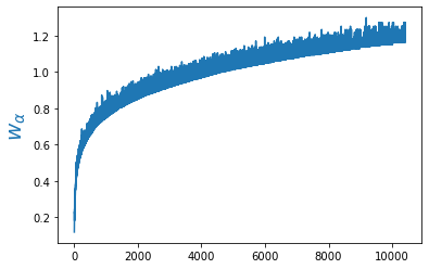
criterion = nn.CrossEntropyLoss(weight = weight)As a result, for example, the loss contribution of the word "the" will be multiplied by 0.12, the word "cat" by 0.62, and "zeus" by 1.27. The figure above shows the weights as a function of the word index in the vocabulary.
The weights are normalized so that their sum equals the vocabulary size V_DIM. This allows approximate comparison between the loss without weights (where all weights equal 1) and the loss with weights. However, it should be remembered that these losses (even for the same model) will differ. Without weights the loss is usually smaller, since the model only needs to learn to predict very frequent words. For example, the token "." has pm = 97442, i.e. its probability is roughly 0.1. If the model always predicts a period, it would already achieve an accuracy of about 0.1.
Training Skip-gram Softmax
One training epoch with 100 samples per batch and a total of 45'671'880 samples takes about one and a half hours on a CPU. Therefore, it is advisable to use a graphics processor unit (GPU) for training.
cpu = torch.device("cpu")
gpu = torch.device("cuda:0" if torch.cuda.is_available() else "cpu")

model.to(gpu)
weight = weight.to(gpu)
Accordingly, during each training loop the batch data must also be transferred to the GPU:
xb = torch.from_numpy( X[it: it+batch_size] ).to(GPU)
yb = torch.from_numpy( Y[it: it+batch_size] ).to(GPU)

y = self.model(xb)
With this setup, one epoch takes about 20 minutes.
For the ROC Stories dataset, the initial loss is approximately 9.41, both with and without weights. The trained model achieves loss=7.3 with weights, and 5.3 without weights. A similar situation occurs with accuracy (when multiplied by the weights).
Skip-gram Negative Sampling
A faster variant is called skip-gram with negative sampling. To account for the asymmetry of the pair $[\mathbf{u},\mathbf{v}]$, we use different embedding vectors for them. We compute their dot product and pass it through a sigmoid function: $$ p = \frac{1}{1+e^{-\mathbf{u}\cdot\mathbf{v}'}}. $$
Below is an implementation of this model in PyTorch using a functional style:
class Skip_gram_Negative1(nn.Module):
    def __init__(self, V_DIM, E_DIM):
        super(Skip_gram_Negative1, self).__init__()

        self.emb1 = nn.Embedding(V_DIM, E_DIM, scale_grad_by_freq=True)
        self.emb2 = nn.Embedding(V_DIM, E_DIM, scale_grad_by_freq=True)

    def forward(self, x):                            # X has two columns
        u  = nn.Flatten() ( self.emb1(x[:,0]) )
        v  = nn.Flatten() ( self.emb2(x[:,1]) )

        dot = u.mul_(v).sum(dim=1)
        return torch.sigmoid(dot)                    # use BCELoss
Another way to account for "asymmetry" is to use a single embedding and rotate the second vector: $\mathbf{v}'=\mathbf{v}\cdot\mathbf{W}$. For this, the vector is passed through a trainable Linear layer with weight matrix $\mathbf{W}$ of shape (E, E). Then we compute the sigmoid of the cosine-like similarity between the vectors. Thus, the probability that vectors $\mathbf{u}$ and $\mathbf{v}$ are neighbors becomes: $$ p = \frac{1}{1+e^{-\mathbf{u}\cdot\mathbf{W}\cdot\mathbf{v}}}. $$ For vectors $(\mathbf{u},\mathbf{v})$ from the same context (parallel vectors) $p\sim 1$, while for vectors from different contexts $p\sim 0$ (both vectors are taken from the same Embedding layer). The trainable matrix $\mathbf{W}$ plays the role of "a metric tensor" when computing the dot product.
class Skip_gram_Negative2(nn.Module):
    def __init__(self, V_DIM, E_DIM):
        super(Skip_gram_Negative2, self).__init__()

        self.emb = nn.Embedding(V_DIM,E_DIM, scale_grad_by_freq=True)
        self.fc  = nn.Linear   (E_DIM, E_DIM)

    def forward(self, x):
        u  = nn.Flatten() ( self.emb(x[:,0]) )
        v  = nn.Flatten() ( self.emb(x[:,1]) )

        dot = (u * self.fc(v)).sum(dim=1)
        return torch.sigmoid(dot)                    # use BCELoss
The main problem with Skip-gram using softmax is that for each training pair we must compute dot products $\mathbf{u}\mathbf{w}_i$ with all words in the vocabulary. And this is a rather time-consuming task. Multiplying matrices (N,E).(E,V) = (N,V) and then computing sum exp (N,V) requires approximately N*V*2*E operations.
(N,E).(E,V)     -> sum exp (N,V)

(N,E)*(N,E).sum -> exp (N)           2*N*E
CBOW
In the simplest version of the CBOW method, the vectors of the context words entering the model are averaged. The resulting mean vector is passed through the weight matrix of a Linear layer with V_DIM neurons and then through the Softmax function (in PyTorch this is not required if the loss CrossEntropyLoss is used). In this case the probabilities of the predicted word are $p_i = e^{\mathbf{u}\mathbf{w}_i}/\sum_j e^{\mathbf{u}\mathbf{v}_j},$ where $\mathbf{u}$ is the average vector of the context words.
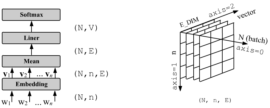
To the right of the network architecture, the tensor shape after the Embedding layer is shown. The model in PyTorch is:
class SBOW(nn.Module):
    def __init__(self, V_DIM, E_DIM):
        super(SBOW, self).__init__()

        self.emb = nn.Embedding(V_DIM,E_DIM, scale_grad_by_freq=True)
        self.fc  = nn.Linear   (E_DIM, V_DIM)

    def forward(self, x):
        x = self.emb(x)
        x = torch.mean(x, dim=1)
        x = self.fc (x)
        return x                              # use CrossEntropyLoss
The model contains 2,011,005 parameters (1,000,500 in Embedding and 1,010,505 in Linear). The number of context words does not affect the number of parameters.
When preparing the data, for the target output $Y$
of each example only the word index (N, ) is specified
(sparse encoding) and the loss torch.nn.CrossEntropyLoss() is used.
Accordingly, for a window with n = 2*WIN inputs,
the inputs also consist of integer indices with shape (N, n).
Vector averaging can be performed with different weights and made trainable. For this purpose, instead of simple averaging we insert a hidden fully connected layer with HIDDEN outputs and the relu activation function:
import torch.nn.functional as F

class SBOW_Hidden(nn.Module):
    def __init__(self, V_DIM, E_DIM, HIDDEN, INPUTS):
        super(SBOW_Hidden, self).__init__()

        self.emb = nn.Embedding(V_DIM, E_DIM, padding_idx=0, scale_grad_by_freq=True)
        self.fc1  = nn.Linear  (INPUTS*E_DIM, HIDDEN)
        self.fc2  = nn.Linear  (HIDDEN, V_DIM)

    def forward(self, x):
        x = self.emb(x)
        x = nn.Flatten()(x)
        x = self.fc1(x)
        x = F.relu(x)
        x = self.fc2(x)
        return x                                # use CrossEntropyLoss

model = SBOW_Hidden(V_DIM, 100, 100, 2*WIN)
Word2Vec and semantic analogies
- Rogers A,... "The (Too Many) Problems of Analogical Reasoning with Word Vectors", (2017)
- Linzen T, "Issues in evaluating semantic spaces using word analogies" (2016)
- Finley G.P.,... "What Analogies Reveal about Word Vectors and their Compositionality" (2017)
Comparison of methods
