ML: Attention - Attention Mechanism
Introduction
The Attention mechanism is currently found in a wide variety of architectures and tasks (translation, text generation, image captioning, etc.). In this document we will consider the historically first use of Attention in the machine translation task (Bahdanau D., et al., 2014) and the implementation of the multi-head attention function in PyTorch. The following documents are devoted to the application of this mechanism in the Transformer network and its development in the GPT and BERT models.
Core Idea
Before diving into technical details, let us consider the idea of the attention mechanism using the example of the task of resolving semantic ambiguity. When working with natural language, each word in the vocabulary is assigned a vector with real-valued components (word embedding). These vectors are fed into a neural network with one architecture or another. The components of the vectors are parameters that are adjusted during training so that words close in meaning have similar vectors. Cosine similarity (the angle between vectors), which is determined by their dot product, is usually used as a measure of closeness.
One of the problems that arises when building word embeddings is the ambiguity of natural language (table - table or spreadsheet, etc.). When training on a corpus of texts, the embedding vector of each word receives fixed components that do not depend on the meaning in which this word appeared in the text.
The attention mechanism (more precisely, self-attention in this case) modifies the embedding vector of each word by "mixing" into it the vectors of its surroundings (context) with certain weights. Suppose, for example, in the sentence "The table has a lot of data" the words correspond to vectors $\mathbf{v}_1,...,\mathbf{v}_7$. To modify the vector $\mathbf{v}_\text{table}=\mathbf{v}_2$, we compute its dot products with other words: $\{w_1,w_2,...,w_7\}=\{\mathbf{v}_2\mathbf{v}_1,~\mathbf{v}_2\mathbf{v}_2,~...,\mathbf{v}_2\mathbf{v}_7\}$ (including itself). We normalize the resulting weights using the softmax function, so that their sum equals one, and the values lie in the range $[0...1]$: $$ w'_i = \text{softmax}(w_1,...,w_7) = e^{w_i}/(e^{w_1}+...+e^{w_7}). $$ The closer to one the weights $w'_i$, the more similar the word $\mathbf{v}_2$ is to the word $\mathbf{v}_i$. Now we construct a new embedding of the word table as a weighted sum: $$ \mathbf{v}'_2 = w'_1\,\mathbf{v}_1+w'_2\,\mathbf{v}_2+...+w'_7\,\mathbf{v}_7. $$ Since articles and prepositions in the vector space are far from the vectors table and data, we will get something like: $$ \begin{array}{llll} \mathbf{v}'_\text{table}\approx 0.9\cdot \mathbf{v}_\text{table}+0.1\cdot \mathbf{v}_\text{data} &~~~~~~~& \text{The table has a lot of data}\\ \mathbf{v}'_\text{table}\approx 0.8\cdot \mathbf{v}_\text{table}+0.2\cdot \mathbf{v}_\text{plate} && \text{There is a plate on the table} \end{array} $$ For text with a different context (the second example above) the components will be different. In the first case, the "attention" of the word table focuses on the word data, and in the second - on the word plate. As a result, a single vector $\mathbf{v}_\text{table}$ common to all meanings splits into two vectors that tend to move towards their semantic clusters (row, digits,... in the first case and chair, furniture, ... - in the second).
Encoder-Decoder
Recall that the simplest Encoder-Decoder architecture consists of two different recurrent networks (encoder and decoder). The encoder receives text in one language (source) as input, and the decoder must output a translation - text in another language (target). The last RNN cell of the encoder at the output contains a vector of hidden state $\mathbf{h}_e^{\text{last}}$, which has "accumulated" information about the entire source sentence (context vector). This vector is sent as the initial hidden state to the first RNN cell of the decoder:
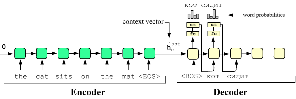
Then the service token <BOS> (begin of sentence) is fed to the input of the first decoder cell. The network is trained to output the translation word "cat" at the output of this cell (see figure). For this, the outputs of the cells are passed through a linear layer (fc) with the number of neurons equal to the number of words in the vocabulary. Then the softmax function (sm) outputs "probabilities" of words from which the number of the maximum is selected (argmax). The vector of the resulting word "cat" is passed to the input of the second cell, and so on until the service token <EOS> (end of sentence) is obtained.
You can also use the teacher forcing method. In this case, the correct translation is fed to all decoder inputs at once, and at the output it is required to output the same sentence shifted one word to the left:
<BOS> cat sits on the mat -> [Decoder] -> cat sits on the mat <EOS>Usually, random switching is performed between the "honest" and "forced" training modes.
The main problem of such an architecture is that with long source sentences the final hidden state of the encoder "forgets" the beginning of the sentence. This problem can be partially solved using bidirectional RNNs. However, even in this case, the hidden state fed to the decoder input poorly "remembers" the middle of the source sentence. A similar problem arises in the decoder, which over time "forgets" the source sentence passed to it (as the hidden state of the last encoder cell). This problem can be reduced by mixing this hidden state into the hidden states of all decoder cells. Other tricks for dealing with long sentences were also invented. However, the most effective turned out to be the attention mechanism.
Attention Focus in RNN
Usually when translating, a person reviews the source sentence several times, focusing on the words important at the given moment and their surroundings, thereby removing syntactic or semantic ambiguity. For example, the word "mat" can mean "rug" or "sports mat". To produce the correct translation, it is necessary to focus not only on the word "mat", but also on the word "cat".
The implementation of this idea is as follows. A weighted sum of all hidden states of the encoder is added to the next hidden state of the decoder. The weight values in the sum reflect the degree of importance of a particular word in the source sentence for generating the current word of the target sentence.
We will denote the hidden state vector of the encoder cell with number $\alpha$ as $\mathbf{v}_{\alpha}=\{v_{\alpha,0},...,v_{\alpha,E-1}\}$, and the decoder as $\mathbf{u}_\alpha=\{u_{\alpha,0},...,u_{\alpha,E-1}\}$, where E is the embedding dimension. The attention weights of the decoder cell number $\alpha$ on the $\beta$-th word of the encoder will be denoted as $w_{\alpha\beta}$. The next $(\alpha+1)$ decoder cell will receive not the current hidden state $\mathbf{u}_\alpha$, but its sum with the weighted hidden states of the encoder $\mathbf{u}_\alpha +\mathbf{u}'_\alpha$, where: $$ \mathbf{u}'_\alpha = \sum_\beta w_{\alpha\beta} \,\mathbf{v}_\beta,~~~~~~~~~~~\sum_\beta w_{\alpha\beta} = 1,~~~~~~~~~~~ w_{\alpha\beta} = f\bigr(\mathbf{u}_\alpha, \mathbf{v}_\beta \bigr). $$ The function $f$ that computes the attention weights $w_{\alpha\beta}$ can be a fully connected layer or a dot product $\mathbf{u}_\alpha\cdot \mathbf{v}_\beta$ (vectors of close words are parallel). Below in the figure, the function $f$ is depicted as a blue circle. The sum of weights $w_{\alpha\beta}$ by the second index $\beta$ must equal one, which is provided by the softmax layer. The hidden states $v_\alpha$, as usual, go both to the output (to the function $f$) and to the next cell of the recurrent layer:
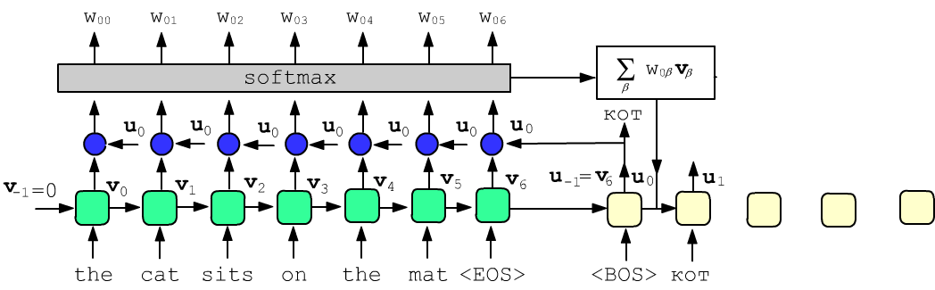
In this example, the hidden state vector obtained when feeding the service word "<BOS>" (begin of sentence) and the last hidden state of the encoder should be closest to the vectors of the first encoder cells (for syntactically similar languages). The vector of the word sits is also mixed into it, and with smaller weights the following words of the source sentence. The second decoder cell, having received the vector of the word "cat" as input, should focus on the word "cat" and semantically close words ("sits", etc.).
We emphasize that source and target languages have different embeddings. However, during training, the vectors of the words "cat" and cat turn out to be close, which leads to an increase in the corresponding attention weights.
If the function $f$ is proportional to the dot product of vectors ($\mu=\text{const}$): $$ f(\mathbf{u},\mathbf{v}) = \mu\,\mathbf{u}\cdot\mathbf{v}, $$ then the attention weights to the decoder hidden states are determined as follows: $$ w_{\alpha\beta} = \text{softmax}\bigr(\mu\,\mathbf{u}_\alpha\mathbf{v}_\beta\bigr) = \frac{e^{\mu\,\mathbf{u}_\alpha\mathbf{v}_\beta} } {\sum_\gamma e^{\mu\, \mathbf{u}_\alpha\mathbf{v}_\gamma } }. $$
Another variant of the weight calculation function contains two matrices $\mathbf{W}_1$, $\mathbf{W}_2$ and a vector $\mathbf{b}$ (whose components are adjusted during training): $$ f(\mathbf{u},\mathbf{v}) = \tanh\bigr(\mathbf{u}\cdot\mathbf{W}_1+\mathbf{v}\cdot\mathbf{W}_2\bigr)\,\mathbf{b}. $$
As weights we will further use the dot product $\omega_{\alpha\beta} = \mu\,\mathbf{u}_\alpha\cdot\mathbf{v}_\beta$ and write the result of the attention mechanism in matrix form.
Attention Function
Suppose there are three matrices: the query matrix $\mathbf{Q}$, the key matrix $\mathbf{K}$ and the value matrix $\mathbf{V}$. The introduced matrices are arguments of the attention function: $$ \mathbf{A} = \text{Attn}( \mathbf{Q},\, \mathbf{K},\, \mathbf{V}) ~=~ \text{softmax} \Bigr(\frac{\mathbf{Q}\cdot\mathbf{K}^\top}{\sqrt{E}}\Bigr)\,\mathbf{V}, $$ where $\top$ is the transpose operation that swaps the indices of the matrix and the softmax function is applied independently to each row of the matrix $\mathbf{Q}\cdot\mathbf{K}^\top/\sqrt{E}$. In the general case, the matrices can have the following shapes: $$ \mathbf{Q}:~~~(N,\,E),~~~~~~~~~~~\mathbf{K}:~~~(M,\,E),~~~~~~~~~~~\mathbf{V}:~~~(M,\,E'),~~~~~~~~~~~\mathbf{A}:~~~(N,\,E'). $$
The names of the introduced matrices are related to a simple associative memory model. We will assume that $M$ pairs of key-value vectors are stored in memory: $(\mathbf{k}_1,\mathbf{v}_1)$,...., $(\mathbf{k}_M,\mathbf{v}_M)$. They are the rows of the matrices $\mathbf{K}$ and $\mathbf{V}$, having, generally speaking, different dimensions $E$ and $E'$. Suppose the query matrix $\mathbf{Q}$ consists of one row ($N=1$) — a vector $\mathbf{q}$ of dimension $E=2$ and there are $M=3$ keys $k_{\alpha i}$ (the first index is the key number, the second is the component number). Then: $$ \mathbf{Q}\,\mathbf{K}^\top ~=~ \begin{array}{|c|c|}\\ \hline q_0 & q_1 \\ \hline \end{array} \cdot \begin{array}{|c|c|}\\ \hline k_{00} & k_{00} \\ \hline k_{10} & k_{10} \\ \hline k_{20} & k_{20} \\ \hline \end{array}^{~\top} ~=~ \begin{array}{|c|c|}\\ \hline q_0 & q_1 \\ \hline \end{array} \cdot \begin{array}{|c|c|c|}\\ \hline k_{00} & k_{10} & k_{20}\\ \hline k_{01} & k_{11} & k_{21}\\ \hline \end{array} ~=~ \begin{array}{|c|c|}\\ \hline \mathbf{q}\mathbf{k}_0 & \mathbf{q}\mathbf{k}_1 & \mathbf{q}\mathbf{k}_2\\ \hline \end{array} $$ If the query vector $\mathbf{q}$ is parallel to the $i$-th key $\mathbf{k}_i$ and anti-parallel to the other keys $\mathbf{q}\mathbf{k}_j \ll -1$, $j\neq i$, then softmax will return a vector of zeros, except for the $i$-th position, where there will be 1. Accordingly, the Attn function will return the value $\mathbf{v}_i$ from the $i$-th pair. In the general case, if there is no exact match between key and query, a weighted sum is returned with a predominance of values whose keys are most similar (co-directed) to the query.
In accordance with the shapes of the matrices $\mathbf{Q},\,\mathbf{K}$, the argument of the softmax function is a matrix of shape $(N,M)$, because $(N,E) \cdot (M,E)^\top= (N,E) \cdot (E,M) = (N,M)$. The softmax function, applied to each row of this matrix (by dimension $M$), gives a matrix $\Omega_{ij}$ of the same shape. The sum of its elements by the second index $j$ equals one for each $i$. This matrix is contracted with $\mathbf{V}$, so the result of the function will be a matrix of shape $(N,\,E')$. If $N > 1$, then the $\text{Attn}$ function simultaneously processes several queries (rows of the $\mathbf{Q}$ matrix).
☝ The matrix inverse to the matrix $\mathbf{A}$ is denoted as $\mathbf{A}^{-1}$, The matrix product $\mathbf{Q}\cdot\mathbf{K}^\top$ of queries and keys, following Vaswani A., et al. (2017), is usually divided by the square root of the dimension $E$ of the vectors of the matrices $\mathbf{Q}$ and $\mathbf{K}$. The motivation for this may be as follows. Suppose the components of two vectors $\mathbf{q}$ and $\mathbf{k}$ are independent random variables with zero mean and unit variance. Then the dot product $\mathbf{q}\cdot\mathbf{k}$ also has zero mean and variance equal to the dimension of the vectors $E$, i.e. typical values $\mathbf{q}\cdot\mathbf{k}$ are in the range $\pm\sqrt{E}$. Scaling translates them to the range $\pm 1$.
Now let us return to the attention mechanism described in the previous section. Let $\mathbf{U}= u_{\alpha i}$ be the hidden state vectors of the decoder, and $\mathbf{V}= v_{\alpha i}$ be the encoder, where the first index is the vector number, and the second is its components (each row of the matrices $\mathbf{U}$ and $\mathbf{V}$ is the $\alpha$-th vector). Then the components of the vectors $\mathbf{u}'_\alpha$ — additions to the decoder hidden state are the rows of the matrix ($\mu = 1/\sqrt{E}$): $$ \mathbf{U}' = \text{Attn}( \mathbf{U},\, \mathbf{V}, \, \mathbf{V}). $$ In this case, $M$ is the number of encoder cells ( = the number of words in the input sentence = the number of key-value pairs), and $N=1$ (one word of the current decoder cell).
The implementation of the Attn function in PyTorch looks as follows (B - batch size, E - embedding dimension, N - number of queries; M - number of key-value pairs):
import math
import torch
import torch.nn as nn

def Attn(Q, K, V):                                        # Q: (B,N,E); K,V: (B,M,E)
    E = Q.size(-1)                                        # embedding dimension E
    W = torch.bmm(Q, K.transpose(-2, -1)) / math.sqrt(E)  # (B,N,M)
    W = nn.functional.softmax(W, dim = -1)                # along the last index of the tensor
    return torch.bmm(W, V)                                # (B,N,E)
The bmm method multiplies two matrices: bmm( (B,N,E), (B,E,M) ) = (B,N,M) independently for each example in the batch, i.e. in a "loop" over examples B multiplies in the usual way: (N,E) @ (E,M) = (N,M).
Self-Attention
The attention mechanism can be applied not only in the encoder-decoder architecture. Consider, for example, the problem of ambiguity of word meanings mentioned at the beginning of the document. Suppose there is a simple network architecture with $N$ inputs and $N$ outputs. $N$ words (in the form of $E$-dimensional embedding vectors) are fed to its inputs, and modified vectors of the same words, taking into account the context of the entire sentence, should be obtained at the outputs.
Let the matrix $\mathbf{V}$ of dimension $(N,E)$ contain $N$ word vectors of the sentence in $N$ rows. Let us compute the value of the function $\text{Attn}(\mathbf{V},\, \mathbf{V},\,\mathbf{V})$. Since the query matrix coincides with the key and value matrices, this situation is called self-attention (self-attention). Let us write the matrix multiplications explicitly, for example, for $N=3$ and $E=2$ (in the matrix $\mathbf{V}:~v_{\alpha i}$, where, as before, the first index is the word number, the second is the component number of its vector): $$ \mathbf{V}\cdot\mathbf{V}^\top ~=~ \begin{array}{|c|c|}\\ \hline v_{00} & v_{01} \\ \hline v_{10} & v_{11} \\ \hline v_{20} & v_{21} \\ \hline \end{array} \cdot \begin{array}{|c|c|}\\ \hline v_{00} & v_{10} & v_{20} \\ \hline v_{01} & v_{11} & v_{21} \\ \hline \end{array} = \begin{array}{|c|c|c|}\\ \hline \mathbf{v}_0\mathbf{v}_0 & \mathbf{v}_0\mathbf{v}_1 & \mathbf{v}_0\mathbf{v}_2 \\ \hline \mathbf{v}_1\mathbf{v}_0 & \mathbf{v}_1\mathbf{v}_1 & \mathbf{v}_1\mathbf{v}_2 \\ \hline \mathbf{v}_2\mathbf{v}_0 & \mathbf{v}_2\mathbf{v}_1 & \mathbf{v}_2\mathbf{v}_2 \\ \hline \end{array} $$ In the first row of the resulting matrix are the dot products of the vector $\mathbf{v}_0$ of the first word with all other words of the sentence. In the second - similar products of the second word $\mathbf{v}_1$ and so on. The largest (positive) values usually have the diagonal elements of the matrix $\mathbf{v}^2_0$, $\mathbf{v}^2_1$, $\mathbf{v}^2_2$ (with comparable vector lengths). After computing the (row-wise) softmax function, we get something like: $$ \text{Attn}(\mathbf{V},\, \mathbf{V},\,\mathbf{V}) ~=~ \text{softmax}\Bigr(\frac{\mathbf{V}\cdot\mathbf{V}^\top}{\sqrt{2}}\Bigr)\cdot\mathbf{V} ~=~ \begin{array}{|c|c|c|}\\ \hline 0.8 & 0.2 & 0 \\ \hline 0.3 & 0.7 & 0 \\ \hline 0.1 & 0 & 0.9 \\ \hline \end{array} \cdot \begin{array}{|c|c|}\\ \hline v_{00} & v_{01} \\ \hline v_{10} & v_{11} \\ \hline v_{20} & v_{21} \\ \hline \end{array} ~=~ \begin{array}{|l|l|}\\ \hline 0.8\,v_{00} + 0.2\,v_{10} & 0.8\,v_{01} + 0.2\,v_{11} \\ \hline 0.7\,v_{10} + 0.3\,v_{00} & 0.7\,v_{11} + 0.3\,v_{01} \\ \hline 0.9\,v_{20} + 0.1\,v_{00} & 0.9\,v_{21} + 0.1\,v_{01} \\ \hline \end{array} $$ Thus, for three words at the output we get three original vectors to which components of semantically close words from the surroundings are "mixed" (if the embedding was successfully built).
Multi-Head Attention
The next stage in the development of Attention technology was the introduction of several trainable attention foci on "different aspects" of the key sequence. Recall that in convolutional networks the number of secondary features is increased by adding additional filters at the next level of image analysis. Similarly, when processing sequences, $H$ attention foci are introduced, which are called heads (each head "looks in its own direction"): $$ \mathbf{A}~=~\text{MultiHead}(\mathbf{Q}, \mathbf{K}, \mathbf{V}) = \text{Concat}(\mathbf{h}_1,\dots,\mathbf{h}_H)\,\mathbf{W}^O, ~~~~~~~~~~~\mathbf{h}_i = \text{Attn}(\mathbf{Q}\,\mathbf{W}_i^Q,~ \mathbf{K}\,\mathbf{W}_i^K,~ \mathbf{V}\,\mathbf{W}_i^V). $$
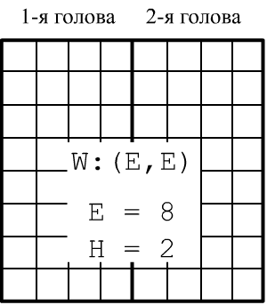
First, linear transformations are performed on the query, key, and value vectors using three matrices $\mathbf{W}^Q_i$, $\mathbf{W}^K_i$, $\mathbf{W}^V_i$. At the same time, for each ($i$-th) head $\mathbf{h}_i$, the set of matrices is its own (its own "attention focus"). If: $$ \mathbf{Q}:~(N,E),~~~~~~~\mathbf{K}:~(M,E_k),~~~~~~~\mathbf{V}:~(M,E_v),~~~~~~~~~~~~\mathbf{A}:~(N,E_a), $$ then, in the general case, the matrices can have the following shapes: $$ \mathbf{W}^Q_i:~(E,\,E_i),~~~~~~~~~~\mathbf{W}^K_i:~(E_k,\,E_i),~~~~~~~~~~\mathbf{W}^V_i:~(E_v,\,E_h),~~~~~~~~\mathbf{h}_i:~(N,\,E_h),~~~~~~~ \mathbf{W}^O:~(E_h\, H,~E_a). $$ After computing the Attn attention function for each head, matrices of shape $(N,E_h)$ are obtained. They are combined into one (concatenated) by the last index, which gives a matrix $(N,~E_h\, H)$. Its contraction with $\mathbf{W}^O$ leads to the final matrix $\mathbf{A}$ of shape $(N,\,E_a)$.
 In the original article (2017), where
attention heads were introduced, it was set $E_i=E_h=E/H$.
The same agreement is adopted in PyTorch
and the matrices of all heads are packed into one with E columns.
For the self-attention task ($E_k=E_v=E$) such a matrix has a square shape $(E,E)$.
$$
\mathbf{W}^Q_i:~(E,\, E/H),~~~~~~~~\mathbf{W}^K:~(E_k,\,E/H),~~~~~~~~~~~~~\mathbf{W}^V_i:~(E_v,\,E/H),~~~~~~~~~~~~\mathbf{W}^O:~(E, ~E).
$$
With this choice, the more heads, the more different aspects of the sequence they can
"see". However, each head "sees worse" because it operates with an embedding of dimension $E/H$.
In the original article (2017), where
attention heads were introduced, it was set $E_i=E_h=E/H$.
The same agreement is adopted in PyTorch
and the matrices of all heads are packed into one with E columns.
For the self-attention task ($E_k=E_v=E$) such a matrix has a square shape $(E,E)$.
$$
\mathbf{W}^Q_i:~(E,\, E/H),~~~~~~~~\mathbf{W}^K:~(E_k,\,E/H),~~~~~~~~~~~~~\mathbf{W}^V_i:~(E_v,\,E/H),~~~~~~~~~~~~\mathbf{W}^O:~(E, ~E).
$$
With this choice, the more heads, the more different aspects of the sequence they can
"see". However, each head "sees worse" because it operates with an embedding of dimension $E/H$.
🔥 Note that in the attention function the elements of the product matrix $\mathbf{W}^Q\cdot\mathbf{W}^{K\top}:~(E,E_k)$ act as parameters, not these two matrices separately. However, if $E_k=E$ and $E_i=E/H$, the number of elements of the two matrices is $2\,E^2/H$, which for three or more heads is less than $E^2$ elements of their product.
MultiheadAttention in PyTorch
In PyTorch there is a ready-made multi-head attention function, formatted as an nn layer:
✒ nn.MultiheadAttention
… (embed_dim, num_heads, dropout=0.0, bias=True, add_bias_kv=False,
… add_zero_attn=False, kdim=None, vdim=None)
The constructor arguments have the following meanings: embed_dim = E - embedding dimension; num_heads = H - number of heads; $\text{kdim}=E_k$, $\text{vdim}=E_v$ - key and value dimensions (if they are None, they are assumed equal to E). The embedding dimension E must be a multiple of the number of heads H. When setting the parameters bias, add_bias_kv to True not only multiplication of queries, keys and values by matrices is performed, but also a shift by a vector (general linear transformation). Forward pass through the attention module has the following parameters:
✒ nn.MultiheadAttention.forward
… (query, key, value, key_padding_mask=None, need_weights=True, attn_mask=None)
In the simplest case, the tensors are fed to the input of the MultiheadAttention object: $\mathbf{Q},~\mathbf{K},~\mathbf{V}$, and at the output a pair ($\mathbf{A}$, $\mathbf{W}$) is obtained — the attention result $\mathbf{A}$ and the weight tensor $\mathbf{W}$ (action of the softmax function for each batch example):
- input: $~~\mathbf{Q}$: (N,B,E), $~~~\mathbf{K},\mathbf{V}$: (M,B,E)
- output: $\mathbf{A}$: (N,B,E), $~~~~~\mathbf{W}$ : (B,N,M),
Note that, by analogy with recurrent layers, the batch example number index B goes not first, but second (except for the resulting weight tensor). Let us give an example of using multi-head attention:
E, H, N, M, B = 100, 10, 3, 3, 1
Ek, Ev        = 100, 100

Q, K, V = torch.rand(N, B, E), torch.rand(M, B, Ek), torch.rand(M, B, Ev)

MHA = nn.MultiheadAttention(E, H, kdim=Ek, vdim=Ev)
A,W = MHA(Q, K, V)

print(tuple(A.shape), tuple(W.shape))               # (3, 1, 100) (1, 3, 3)
The matrix dimensions are: $\mathbf{W}^Q:$ (E, E), $\mathbf{W}^K:$ (E, kdim), $\mathbf{W}^V:$ (E, vdim), where the dimensions kdim,vdim are either set or equal to E (they are passed to the linear function, so they are transposed during multiplication). The dimension of each head is E // H. The output matrix $\mathbf{W}^O:$ is the Linear(E, E, bias=bias) layer.
If the input embeddings are the same, then the projection matrices are packed
in in_proj_weight of shape (3*E,E),
otherwise these are three different matrices: q_proj_weight, k_proj_weight, v_proj_weight.
The bias (if any) is in_proj_bias of shape (3*E,),
and the output layer: out_proj:
for k, v in MHA.state_dict().items():               # in_proj_weight   shape: (300, 100)
    print(f'{k:20s}  shape: {tuple(v.shape)} ')     # in_proj_bias     shape: (300,)
                                                    # out_proj.weight  shape: (100, 100)
                                                    # out_proj.bias    shape: (100,)
Masked Attention
Important parameters of forward pass through the multi-head attention layer are the masks key_padding_mask and attn_mask.
The boolean mask key_padding_mask: (B,M) allows excluding some key-value pairs from the attention mechanism (independently for each batch example B). For this, the numbers of the excluded pairs in the mask must be marked with the value True.
The real-valued mask attn_mask: (N,M) is added to the attention weights before their normalization using the softmax function. Usually this mask is used to selectively disable specific weights. For this, the corresponding elements of the mask are set to minus infinity, and the rest to zero:
E, H, N, M, B = 8, 4, 3, 4, 1
Q, K, V = torch.rand(N,B,E), torch.rand(M,B,E), torch.rand(M,B,E)

MHA = nn.MultiheadAttention(E,H)

A,W = MHA(Q, K, V,
          key_padding_mask=torch.tensor( [[False,True,False,True]]) )
print(W)

inf = float("-inf")
A,W = MHA(Q, K, V,
          attn_mask=torch.tensor( [[inf, 0.0, 0.0, inf],
                                   [0.0, 0.0, 0.0, 0.0],
                                   [inf, 0.0, 0.0, inf]] ) )
print(W)
In the first case key_padding_mask
disabled keys with indices 1 and 3
Below, the corresponding columns of the weight matrix W are filled with zeros.
The attn_mask mask "removed" the corner elements of the attention weight matrix:
[[[0.5148, 0.0000, 0.4852, 0.0000],              [[[0.0000, 0.4940, 0.5060, 0.0000],
  [0.5136, 0.0000, 0.4864, 0.0000],                [0.2570, 0.2519, 0.2435, 0.2475],
  [0.5127, 0.0000, 0.4873, 0.0000]]]               [0.0000, 0.4918, 0.5082, 0.0000]]],
From the document devoted to the transformer, the practical benefit of using these masks will become clear.
MultiheadAttention Implementation
Let us reproduce the computations that occur inside the nn.MultiheadAttention layer. We will need the following PyTorch functions:
from torch               import bmm                   # batch matrix multiplication
from torch.nn.functional import linear  as linear     # linear function y = x@A^T + b
from torch.nn.functional import softmax as softmax    # softmax function
In the MultiHeadAttention function, in addition to the query Q, key K, value V matrices and masks key_mask, attn_mask, we will also pass the linear transformation matrices, which we will take from the nn.MultiheadAttention layer. In the comments, as usual, the shapes of the resulting tensors are given:
def MultiHeadAttention(Q,K,V,                         # Q:(N,B,E);  K:(M,B,Ek);  V:(M,B,Ev)
                       Wq, Wk, Wv, Wo,                # rotation matrices for Q,K,V,A
                       Bq=None, Bk=None, Bv=None, Bo=None,  # bias matrices for Q,K,V,A
                       key_mask  = None,              # key exclusion mask (B,M)
                       attn_mask = None):             # additive mask        (N,M)

    q = linear(Q, Wq, Bq)                             # (N,B,E) linear transformation
    k = linear(K, Wk, Bk)                             # (M,B,E)
    v = linear(V, Wv, Bv)                             # (M,B,E)

    q = q.view(N, B*H, E//H).transpose(0,1)           # (B*H, N, E/H)  split into H heads
    k = k.view(M, B*H, E//H).transpose(0,1)           # (B*H, M, E/H)
    v = v.view(M, B*H, E//H).transpose(0,1)           # (B*H, M, E/H)

    W = bmm(q, k.transpose(1,2))*float(E//H)**-0.5    # (B*H, N, M) head dimension E/H

    if attn_mask is not None:                         # additive mask
        W += attn_mask.unsqueeze(0)                   # (N,M) -> (1,N,M)

    if key_mask is not None:                          # exclude part of the keys
        W = W.view(B, H, N, M)
        key_mask = key_mask.unsqueeze(1).unsqueeze(2) # (B,1,1,M)
        W = W.masked_fill(key_mask, float('-inf'))
        W = W.view(B*H, N, M)

    W = softmax(W, dim=-1)                            # (B*H, N, M)

    A = bmm(W, v)                                     # (B*H, N,  E/H)

    A = A.transpose(0, 1).contiguous().view(N,B,E)    # (N, B, E)
    W = W.view(B, H, N, M)
    return linear(A, Wo, Bo), W.sum(dim=1) / H        # (N, B, E), (B, N, M)
First, Q, K, V undergo linear transformation linear. Then they are split into heads. For this, their shape is changed and the first two indices are swapped. As a result, the first index numbers both examples and heads. Using the bmm multiplication method further performs multiplication of rectangular matrices for each example, each head. Transposition and shape change of the tensor A at the end of the function translates it into the original shape, similar to the tensor Q.
In the if blocks, attention masking occurs. First, the attn_mask mask is added to the weights W, to which one dimension is added (and then the broadcasting mechanism is enabled). Then the boolean mask key_mask serves to replace the columns for which key_mask == True with minus infinity. After passing through the softmax function, the elements of the weight matrix in these columns will be equal to zero.
If the MHA object is created using the nn.MultiheadAttention constructor (as in the previous section), then the call to the written function will look as follows:
A2,W2 = MultiHeadAttention(Q,K,V,
                           MHA.in_proj_weight[0 : E]   if Ek==E else  MHA.q_proj_weight,
                           MHA.in_proj_weight[E : 2*E] if Ek==E else  MHA.k_proj_weight,
                           MHA.in_proj_weight[E*2 : ]  if Ek==E else  MHA.v_proj_weight,
                           MHA.out_proj.weight,
                           MHA.in_proj_bias[0 : E],
                           MHA.in_proj_bias[E : E*2],
                           MHA.in_proj_bias[E*2:],
                           MHA.out_proj.bias,
                           attn_mask = attn_mask,
                           key_mask = key_mask  )

print(((A1.detach() - A2.detach())**2).sum()**0.5)   # compare matrices (rounding)
print(((W1.detach() - W2.detach())**2).sum()**0.5)
References
Articles
- 2014: Sutskever I, et al. "Sequence to Sequence Learning with Neural Networks"
- invention of the Encoder-Decoder architecture for RNN. - 2014: Bahdanau D., et al. "Neural Machine Translation by Jointly Learning to Align and Translate
- Attention mechanism for Encoder-Decoder architecture. - 2017: Vaswani A., et al. "Attention is All You Need"
- abandonment of recurrent networks, Transformer architecture (Google Brain)
Sources
- The Annotated Encoder-Decoder with Attention
- NLP From Scratch: Translation with a Sequence to Sequence Network and Attention
- The Annotated Transformer - analysis of transformer code.
- "Attention and Augmented Recurrent Neural Networks"
