ML: Recurrent Networks in PyTorch
Introduction
Sometimes the training data consists of ordered sequences. Examples include time series (stock prices, sensor readings) or natural language text. In these cases, recurrent neural networks (RNNs) are the appropriate architecture.
We will be using the PyTorch framework, the basics of which you can learn here and here. Importing its libraries looks like this:
import torch
import torch.nn as nn
All examples are in the file ML_RNN_Torch.ipynb, and the discussion of recurrent networks using the Keras library is provided here.
Simple RNN
A recurrent layer consists of L cells with identical parameters.
An ordered sequence of length L is fed into it: $\mathbf{x}^{(0)},...,\mathbf{x}^{(\mathrm{L}-1)}$.
The elements of the sequence are E-dimensional feature vectors
$\mathbf{x}^{(t)}=\{x^{(t)}_0,...,x^{(t)}_{\mathrm{E}-1}\}$
(E comes from word embedding).
The first vector is fed to the first cell, the second to the second cell, and so on.
Each cell is characterized by an H-dimensional hidden state vector
$\mathbf{h}=\{h_0,...,h_{\mathrm{H}-1}\}$.
This vector is the output of the cell (upward arrow)
and is also sent to the next cell. Inside a simple RNN cell
the following computation is performed (for $t=0,...,\text{L}-1$):
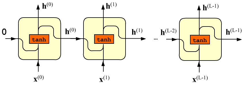
The matrices $\mathbf{W}:$(E, H), $~\mathbf{H}:$(H, H) and the vector $~\mathbf{b}:$(H,) are the parameters of the cell (and the entire layer). Since the cells are identical, the number of inputs L does not affect the number of parameters. The total number of parameters is (E + H + 1) * H. The initial hidden state vector $\mathbf{h}^{(-1)}$ (entering the first cell) is either a zero vector $\mathbf{0}$ or is set manually.
The nonlinear hyperbolic tangent function $\tanh(x)=(e^x-e^{-x})/(e^x+e^{-x})$ is necessary, as usual, so that the sequence of matrix multiplications does not "collapse" into one. The sign-alternating nature of tanh fights uncontrolled positive growth of the components of the vector $\mathbf{h}^{(t)}$ during sequential (recurrent) matrix multiplications.
Examples of RNN architectures
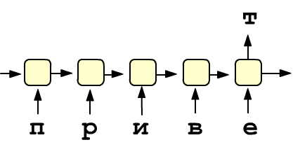 The hidden state vector gradually "accumulates" averaged information about previous inputs.
The final vector $\mathbf{h}^{(\mathrm{L}-1)}$ characterizes the entire sequence and is called
the context vector.
It can, for example, be fed into a stack of linear layers,
at the output of which text classification occurs (sentiment analysis - positive or negative product review)
or the next member of the sequence is predicted. On the right is an example of a simple architecture
that predicts the next letter in the text. Additional layers are assumed to be present.
The hidden state vector gradually "accumulates" averaged information about previous inputs.
The final vector $\mathbf{h}^{(\mathrm{L}-1)}$ characterizes the entire sequence and is called
the context vector.
It can, for example, be fed into a stack of linear layers,
at the output of which text classification occurs (sentiment analysis - positive or negative product review)
or the next member of the sequence is predicted. On the right is an example of a simple architecture
that predicts the next letter in the text. Additional layers are assumed to be present.
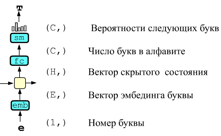 The letter number in the alphabet is fed into the Embedding vectorization layer.
At its output, an E-dimensional vector is obtained, the components of which are training parameters.
After passing through the RNN cell, this vector changes its dimensionality,
turning into an H-dimensional vector of new features at the cell output.
Then it is sent to a regular fully connected layer with "C" neurons,
where "C" equals the number of letters in the alphabet.
Passing this C-dimensional vector through the softmax function
gives the "probabilities" of the next letter in the sequence. The training task is to select the parameters
of the RNN cell and the embedding vectors so that the probability of predicting
the correct letter is maximized.
The letter number in the alphabet is fed into the Embedding vectorization layer.
At its output, an E-dimensional vector is obtained, the components of which are training parameters.
After passing through the RNN cell, this vector changes its dimensionality,
turning into an H-dimensional vector of new features at the cell output.
Then it is sent to a regular fully connected layer with "C" neurons,
where "C" equals the number of letters in the alphabet.
Passing this C-dimensional vector through the softmax function
gives the "probabilities" of the next letter in the sequence. The training task is to select the parameters
of the RNN cell and the embedding vectors so that the probability of predicting
the correct letter is maximized.
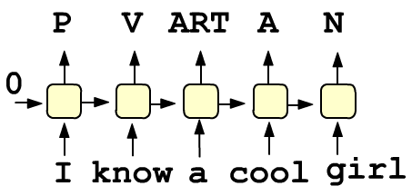 You can use not only the last hidden state, but also the hidden states of all cells.
For example, the architecture of a network that performs text labeling, where each word is assigned its part of speech (pronoun,
verb, article, adjective, noun) looks like the one shown on the right.
As in the previous example, embedding layers for words must be present on all inputs.
At the output — a fully connected layer with the number of neurons equal to the number of parts of speech and a softmax function giving their probabilities.
You can use not only the last hidden state, but also the hidden states of all cells.
For example, the architecture of a network that performs text labeling, where each word is assigned its part of speech (pronoun,
verb, article, adjective, noun) looks like the one shown on the right.
As in the previous example, embedding layers for words must be present on all inputs.
At the output — a fully connected layer with the number of neurons equal to the number of parts of speech and a softmax function giving their probabilities.
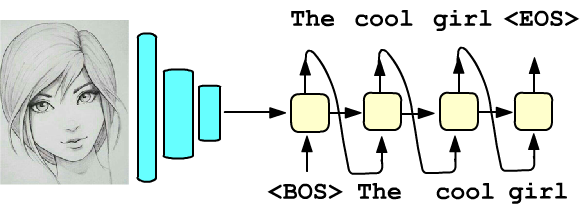 In the examples above, the initial hidden state entering the first cell
was a zero vector.
This vector can also be derivative features of some object. For example,
on the right a schematic representation of the task of generating a textual description of an image is shown.
The pixels of the original image are passed through a sequence of convolutional layers. The weights of these layers are trained
on some other task (for example, object class recognition). The final layer of the convolutional network
is sent as the initial hidden state to the RNN layer.
The input to its first cell is the embedding of the service token (word) <BOS> (begin of sentence).
The recurrent network is trained to output text relevant to the image on its outputs. In this case, the first generated word is fed to the input of the second
cell and so on, until at some iteration the layer outputs the service token <EOS> (end of sentence).
In the examples above, the initial hidden state entering the first cell
was a zero vector.
This vector can also be derivative features of some object. For example,
on the right a schematic representation of the task of generating a textual description of an image is shown.
The pixels of the original image are passed through a sequence of convolutional layers. The weights of these layers are trained
on some other task (for example, object class recognition). The final layer of the convolutional network
is sent as the initial hidden state to the RNN layer.
The input to its first cell is the embedding of the service token (word) <BOS> (begin of sentence).
The recurrent network is trained to output text relevant to the image on its outputs. In this case, the first generated word is fed to the input of the second
cell and so on, until at some iteration the layer outputs the service token <EOS> (end of sentence).
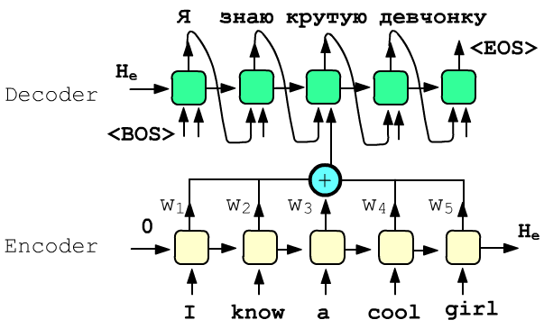 The last example is related to machine translation and the attention architecture.
Suppose there are two recurrent layers with different parameters.
The first is called the encoder (encoder), and the second is the decoder (decoder).
The embeddings of the words of the sentence
"I know a cool girl"
in the source language are fed to the inputs of the encoder cells.
The decoder is expected to output the translation of the sentence into the target language:
"I know a cool girl".
The last example is related to machine translation and the attention architecture.
Suppose there are two recurrent layers with different parameters.
The first is called the encoder (encoder), and the second is the decoder (decoder).
The embeddings of the words of the sentence
"I know a cool girl"
in the source language are fed to the inputs of the encoder cells.
The decoder is expected to output the translation of the sentence into the target language:
"I know a cool girl".
The hidden states of the RNN encoder, as usual, accumulate information about the source sentence. Their sum with certain weights $w_i$ is fed as additional inputs to the cells of the decoder recurrent layer (the figure shows only one such input). The weights are computed by a trainable function of the encoder hidden states and the decoder hidden state from the previous cell (in the example this is "know"). The current decoder hidden state "assumes" what is important in the source sentence for translation and "focuses attention" on the necessary information, which is reflected in the values of the weights $w_i$.
Matrix multiplications
Let's consider how the matrices $\mathbf{x}^{(t)}\cdot \mathbf{W} + \mathbf{h}^{(t-1)}\cdot \mathbf{H} + \mathbf{b}$
are multiplied when computing the hidden state.
In the general case, the current input $\mathbf{x}^{(t)}$ is fed to the RNN cell in batches of
B examples each.
Therefore, the $t$-th feature vector $\mathbf{x}^{(t)}$ is a matrix of shape (B,E)
(the examples are in the rows).
This matrix is multiplied on the left by the matrix $\mathbf{W}:$ (E,H)
and then the product of the matrices $\mathbf{h}^{(t-1)}:$ (B,H)
and $\mathbf{H}:$ (H,H) is added. The bias vector $\mathbf{b}$ is then added:
$$
\underbrace{\text{(B,E)} \cdot \text{(E,H)}}_{\mathbf{x}^{(t)}\,\cdot\,\mathbf{W}} ~~~+~~~
\underbrace{\text{(B,H)}\cdot\text{(H,H)}}_{\mathbf{h}^{(t-1)}\,\cdot\,\mathbf{H}} ~~~+~~~
\underbrace{\text{(1,H)}}_{\mathbf{b}} ~~~=~~~ \text{(B,H)}
$$
Let the input and hidden state dimensions be E=2 and H=3,
and the number of examples in the batch B=4. Then in one cell the following computation occurs,
the result of which is then passed through tanh:
The same can be done more compactly by concatenating the vectors $\mathbf{x}^{(t)}$, $\mathbf{h}^{(t-1)}$ on the right: torch.cat([x,h], dim=1) and attaching the matrix $\mathbf{H}$ to the matrix $\mathbf{W}$ from below: torch.cat([W,H], dim=0):
$$ \begin{array}{|c|c|c|c|c|} \hline x^{(t)\phantom{-1}}_{00} & x^{(t)\phantom{-1}}_{01} & h^{(t-1)}_{00} & h^{(t-1)}_{01}& h^{(t-1)}_{02}\\ \hline x^{(t)\phantom{-1}}_{10} & x^{(t)\phantom{-1}}_{11} & h^{(t-1)}_{10} & h^{(t-1)}_{11}& h^{(t-1)}_{12}\\ \hline x^{(t)\phantom{-1}}_{20} & x^{(t)\phantom{-1}}_{21} & h^{(t-1)}_{20} & h^{(t-1)}_{21}& h^{(t-1)}_{22}\\ \hline x^{(t)\phantom{-1}}_{30} & x^{(t)\phantom{-1}}_{31} & h^{(t-1)}_{30} & h^{(t-1)}_{31}& h^{(t-1)}_{32}\\ \hline \end{array} \cdot \begin{array}{|c|c|c|} \hline W_{00}^{\phantom{(0)}} & W_{01} & W_{02} \\ \hline W_{10}^{\phantom{(0)}} & W_{11} & W_{12} \\ \hline H_{00}^{\phantom{(0)}} & H_{01} & H_{02} \\ \hline H_{10}^{\phantom{(0)}} & H_{11} & H_{12} \\ \hline H_{20}^{\phantom{(0)}} & H_{21}& H_{22} \\ \hline \end{array} ~~+~~ \begin{array}{|c|c|c|} \hline b_{0} & b_{1} & b_{2}\\ \hline \end{array} ~~=~~ \begin{array}{|c|c|c|} \hline r_{00} & r_{01} & r_{02}\\ \hline r_{10} & r_{11} & r_{12}\\ \hline r_{20} & r_{21} & r_{22}\\ \hline r_{30} & r_{31} & r_{32}\\ \hline \hline \end{array} $$
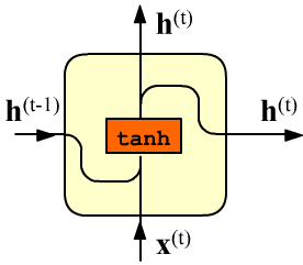 This is why the merged arrows of the vectors $\mathbf{x}^{(t)},\mathbf{h}^{(t-1)}$
are drawn on the input of $\tanh$ in the cell diagram.
This is why the merged arrows of the vectors $\mathbf{x}^{(t)},\mathbf{h}^{(t-1)}$
are drawn on the input of $\tanh$ in the cell diagram.
Such computations are performed in each cell. If the input tensor X
has shape (L,B,E),
then X[t] are matrices of shape (B,E) considered above:
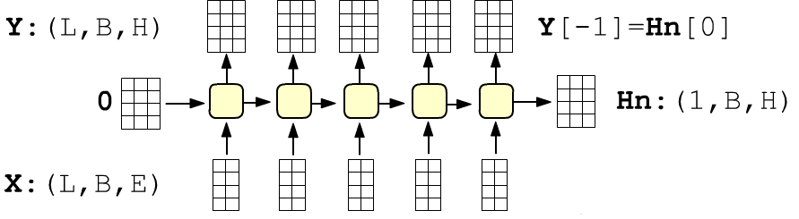
The hidden state of the last cell Hn is conventionally considered to have shape (1,B,H), not (B,H).
Recurrent networks in PyTorch
In PyTorch a simple recurrent layer is called nn.RNN. Its mandatory parameters are the input dimension E and hidden state dimension H:
E, H  = 2, 3                             # input and hidden state dimensions
B, L  = 4, 5                             # number of examples, sequence length (number of vectors)

rnn = nn.RNN(E, H)                       # instance of nn.RNN class
Let's output the names of the RNN layer parameters and their shapes:
for k, v in rnn.state_dict().items():    # weight_ih_l0 : (3, 2)        (H,E)
    print(f'{k:10s} : {tuple(v.shape)}') # weight_hh_l0 : (3, 3)        (H,H)
                                         # bias_ih_l0   : (3,)          (H,)
                                         # bias_hh_l0   : (3,)          (H,)
As in the linear layer, the weight matrices are stored in transposed form for row-wise matrix multiplication. Note that the parameter list contains two bias vectors. In reality, the meaningful parameter is the summed vector bias_ih_l0 + bias_hh_l0. The source code explains that: "Second bias vector included for CuDNN compatibility" (this apparently makes it work faster on graphics cards).
Create a random dataset X and feed it into the recurrent layer. The output will be a tuple: a tensor of all hidden states of shape (L,B,H) and a tensor of the hidden state of the last cell (1,B,H):
X  = torch.rand(L, B, E)
Y, Hn = rnn(X)                           # all outputs and the last hidden state
                                         #  (L, B, H) (1, B, H)
print(tuple(Y.shape), tuple(Hn.shape))   #  (5, 4, 3) (1, 4, 3)   Y[-1] == Hn[0]
Let's reproduce the computations that occur inside a simple recurrent layer. To do this, get the cell parameter values from the rnn object (detached from the graph using the detach method):
W_ih, W_hh = rnn.weight_ih_l0.detach(), rnn.weight_hh_l0.detach()
B_ih, B_hh = rnn.bias_ih_l0.detach(),   rnn.bias_hh_l0.detach()
Fill the hidden state $\mathbf{h}^{(-1)}$ entering the first cell with zeros, as nn.RNN does by default.
Loop through all cells (the addmm(v,M1,M2) method computes v + M1 @ M2):
Hn = torch.zeros(B,H)                    # initial hidden state - zeros

for x in X:                              # for each cell for x:(B,E) in  X:(L,B,E)

    Hn =torch.tanh(  torch.addmm(B_ih, x,  W_ih.t())
                   + torch.addmm(B_hh, Hn, W_hh.t()) )
    print(Hn)
The initial hidden state can be passed to the network object as the second parameter (then it will be non-zero). Repeat the previous computations by feeding one input of the sequence at a time into rnn:
Hn = torch.zeros(1,B,H)                  # initial hidden state - zeros
for x in X:
    _, Hn = rnn( x.view(1,B,E), Hn )     # Hn from the previous cell
    print(Hn)
Bidirectional layer and stacked layers
 Sometimes the present is influenced not only by the past, but also by the future.
For example, the meaning of a word in a sentence is determined by the entire sentence,
and not only by the words preceding it.
Sometimes the present is influenced not only by the past, but also by the future.
For example, the meaning of a word in a sentence is determined by the entire sentence,
and not only by the words preceding it.
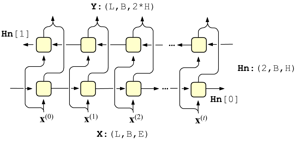
In this case, it is appropriate to use two recurrent layers with different parameters together. In the first layer, hidden states propagate from left to right, and in the second — from right to left. The input vectors are fed independently to each layer, and the layer outputs are concatenated. Therefore, the output tensor has dimensionality (L,B,2*H). The final hidden states in Hn: (2,B,H) come from each layer. In this case Hn[0] is the hidden state of the last (rightmost) cell of the first layer, and Hn[1] is the first (leftmost) cell of the second layer. In PyTorch a bidirectional layer is created as follows:
rnn = nn.RNN(E, H, bidirectional=True)
A recurrent layer (single or bidirectional) can be turned into a stack of layers:
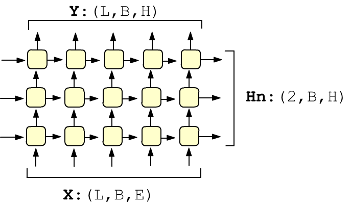 rnn = nn.RNN(E, H, num_layers=3)
Let Dir = 2 if bidirectional==True else 1.
If the number of layers is Num, then
the input and output tensors in the general case have the following shapes:
X :  (L,       B, E)   =>   Y : (L,       B, Dir*H)
H0:  (Num*Dir, B, H)   =>   Hn: (Num*Dir, B,   H  )
Sequence packing
Training sequences often have different lengths. For example, the number of words varies significantly from sentence to sentence. There are various strategies for working with RNN in such situations.
You can feed one sequence at a time into RNN (B=1). Since PyTorch builds dynamic graphs, the required number of cells will be "created on the fly". However, passing one example at a time through the network slows down computations, especially when using graphics cards. If the length variation is small, you can sort the sequences by length and form batches from examples of the same length.
Finally, when forming batches, you can use the function pack_padded_sequence, which itself sorts the examples in the batch in descending order of length and forms the longest possible batch for each cell.
from torch.nn.utils.rnn import pack_padded_sequence, pad_packed_sequenceLet's illustrate the operation of this function with an example. Suppose the batch B=4 contains training examples. The first has length 5, the second — 3, the third — 4 and the fourth — 2. The examples are combined into a tensor; shorter sequences are padded to the maximum length L=5 with zero input vectors (dimension E=2). Thus the input tensor X has shape (L,B,E)=(5,4,2):
X = torch.tensor([[1,1],[1,2],[1,3],[1,4],[1,5],
                  [2,1],[2,2],[2,3],[0,0],[0,0],
                  [3,1],[3,2],[3,3],[3,4],[0,0],
                  [4,1],[4,2],[0,0],[0,0],[0,0]],
                  dtype=torch.float)

X = X.view(B,L,E)          # (B*L,E)->(B,L,E)
X = X.transpose(0,1)       # -> (L,B,E)
Set the lengths of the examples X_len (lengths of the rows if zeros are discarded) and call the packing function:
X_len = torch.tensor([5,3,4,2])# lengths of examples

Xp    = pack_padded_sequence(X, # packing
                             X_len,
                             enforce_sorted=False)
PackedSequence(
data=tensor(
       [[1., 1.],
        [3., 1.],
        [2., 1.],
        [4., 1.],  <- 1st cell B=4
        [1., 2.],
        [3., 2.],
        [2., 2.],
        [4., 2.],  <- 2nd cell B=4
        [1., 3.],
        [3., 3.],
        [2., 3.],  <- 3rd cell B=3
        [1., 4.],
        [3., 4.],  <- 4th cell B=2
        [1., 5.]]),<- 5th cell B=1

batch_sizes    = tensor([4,4,3,2,1]),
sorted_indices = tensor([0,2,1,3]))
Now you can send the packed sequence to the network: Yp, Hn = rnn(Xp). The last hidden state Hn will be the usual size (1,B,H)=(1,4,3). The outputs of all cells Yp, like the inputs Xp, will be packed. To unpack them, you need to call the second function:
Y, Y_len = pad_packed_sequence(Yp)The result will look something like this (now Y[-1] != Hn[0], because Hn contains the last non-zero rows from all outputs Y[i]):
Y[0] = [[-0.4083,  0.2363,  0.8988],     |    Y[-1]= [[-0.8162,  0.9937,  0.9942],
        [-0.8875, -0.6924,  0.9849],     |            [ 0.0000,  0.0000,  0.0000],
        [-0.7268, -0.2967,  0.9605],     |            [ 0.0000,  0.0000,  0.0000],
        [-0.9561, -0.8852,  0.9943]]     |            [ 0.0000,  0.0000,  0.0000]]

Y_len = tensor([5, 3, 4, 2])                             # the same as X_len
The algorithm for working with RNN using packed data is reproduced as follows:
Hn = torch.zeros(Xp.batch_sizes[0], H)                   # zeros in the initial state
Yp = torch.empty(len(Xp.data),      H)                   # packed tensor of cell outputs

beg = 0
for bs in Xp.batch_sizes:                                # for each batch size
    XX = Xp.data[beg: beg + bs]                          # current cell batch
    HH = Hn[ : bs]                                       # hidden state entering it

    HH = torch.tanh(   torch.addmm(B_ih, XX, W_ih.t())   # actual computations
                     + torch.addmm(B_hh, HH, W_hh.t()) )

    Yp[beg: beg + bs].copy_(HH)                          # pack the output batch
    Hn[   :       bs].copy_(HH)                          # accumulate it in the hidden state
    beg += bs
Hn = Hn[Xp.sorted_indices]                               # restore original row order

print(Yp, Hn)                                            # will match Yp, Hn = rnn(Xp)
In addition to input=X and length, the packing functions have two more parameters. If enforce_sorted = True, the batch must be sorted in descending order of sequence lengths. The parameter batch_first = True assumes that the input tensor has shape (B,L,E). This same parameter must then be used in the RNN constructor when creating the layer instance.
All parameters of the RNN class
Here is the full list of parameters of the RNN class in the PyTorch framework:
✒ nn.RNN
… (input_size,
hidden_size, num_layers=1, nonlinearity='tanh', bias=True,
… batch_first=False, dropout=0, bidirectional=False)
[doc]
Note the previously unmentioned parameter dropout. By default it is zero. When non-zero, after each layer (num_layers > 1), except the last one, a dropout layer is inserted, which with probability dropout randomly "turns off" (sets to zero) some elements of the tensors at the output of each cell.
Setting the bias parameter to False removes the bias vector after the matrix multiplication.
LSTM cell
In the LSTM layer (long short-term memory), in addition to the hidden state $\mathbf{h}$ between cells the "cell state" (memory state) $\mathbf{c}$ is also passed. The dimension H of this vector coincides with the dimension of the hidden state $\mathbf{h}$. The vectors $\mathbf{c}$ regulate which features should be remembered or forgotten when passing to the next cell, which improves long-term memory.
Inside the LSTM cell there are four linear layers with H neurons. Three of them have sigmoid activation $\sigma$ (output vector with values $[0...1]$) and one layer with hyperbolic tangent $\tanh$: $[-1...1]$.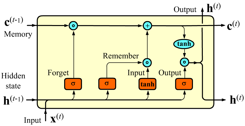
Before this computation, the incoming memory vector $\mathbf{c}^{(t-1)}$ is modified. First, $\mathbf{x}^{(t)}, \mathbf{h}^{(t-1)}$ enter the fully connected Forget layer with sigmoid activation (forget gate). The output dimension of this layer is H (same as $\mathbf{h}$ and $\mathbf{c}$). This vector is multiplied element-wise by the components of the previous memory vector $\mathbf{c}^{(t-1)}$. It is assumed that during multiplication some features in $\mathbf{c}^{(t-1)}$ are forgotten (if multiplied by 0), and some continue (if multiplied by 1). Example of forgetting: "He took gin, and she took martini" ("took" after "she" can forget about "he"). Similarly, a period as a sentence end marker should zero out a significant part of the components of the memory vector $\mathbf{c}^{(t)}$.
A similar mechanism works for the next gate implementing remembering. The features that need to be remembered are added to the vector $\mathbf{c}$. The layer with $\tanh$ [-1...1] forms "candidate features", and the layer with sigmoid [0...1] strengthens or weakens the role of the remembered feature. Analytically, the computations in the LSTM cell look as follows: $$ \left\{ \begin{array}{lclclcl} \mathbf{F} &=& ~~~~~~\sigma(\mathbf{x}^{(t)}\, \mathbf{W}_{f} &+& \mathbf{h}^{(t-1)}\, \mathbf{H}_{f} &+& \mathbf{b}_f),\\ \mathbf{I} &=& ~~~~~~\sigma(\mathbf{x}^{(t)}\, \mathbf{W}_{i} &+& \mathbf{h}^{(t-1)}\, \mathbf{H}_{i} &+& \mathbf{b}_i),\\ \mathbf{R} &=& \text{tanh}(\mathbf{x}^{(t)}\, \mathbf{W}_{r} &+& \mathbf{h}^{(t-1)}\, \mathbf{H}_{r} &+& \mathbf{b}_r),\\ \mathbf{O} &=& ~~~~~~\sigma(\mathbf{x}^{(t)}\, \mathbf{W}_{o} &+& \mathbf{h}^{(t-1)}\, \mathbf{H}_{o} &+& \mathbf{b}_o), \end{array} \right. ~~~~~~~~~~~~~~~~~~ \left\{ \begin{array}{lcl} \mathbf{c}^{(t)} &=& \mathbf{F} \odot \mathbf{c}^{(t-1)} + \mathbf{R}\odot \mathbf{I},\\[2mm] \mathbf{h}^{(t)} &=& \tanh\bigr(\mathbf{c}^{(t)}\bigr) \odot \mathbf{O}. \end{array} \right. $$
The matrix dimensions for E$=\dim(\mathbf{x}),~~$ H$=\dim(\mathbf{h}),~\dim(\mathbf{c})$ are: $$ \mathbf{W}_{i}, ~\mathbf{W}_{f}, ~\mathbf{W}_{r}, ~\mathbf{W}_{o}:~~~\mathrm{(E, H)};~~~~~~~~~~ \mathbf{H}_{i}, ~\mathbf{H}_{f}, ~\mathbf{H}_{r}, ~\mathbf{H}_{o}:~~~\mathrm{(H, H)};~~~~~~~~~~ \mathbf{b}_i, ~\mathbf{b}_f, ~\mathbf{b}_r, ~\mathbf{b}_o: ~~~~\mathrm{(1, H)}. $$ In PyTorch the LSTM network is implemented by the class torch.nn.LSTM. Unlike torch.nn.RNN, the forward pass returns three tensors: Y, Hd, Cn (the hidden state and memory vector have the same dimension).GRU cell
The Gated Recurrent Unit (GRU) is a simplified version of LSTM with comparable computational power. It performs the following computations: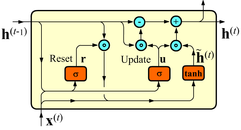
Gradient propagation
Let's consider the features of gradient propagation through the recurrent layer during training. The gradient flow depends heavily on how the loss $L$ that initiates it is computed.
For definiteness, we will predict the next letter in the text.
Suppose the letters are vectorized (embedding)
and fed to the layer input as a sequence of L=5
vectors: $\{\mathbf{x}^{(0)},\mathbf{x}^{(1)},\mathbf{x}^{(2)},\mathbf{x}^{(3)},\mathbf{x}^{(4)}\}$.
The output of the last cell can be fed to a fully connected layer (with the number of neurons equal to the number of letters) and then passed through the
softmax function, which gives the "probabilities" of the next letter $\mathbf{x}^{(5)}$.
In a more general case, the network can be trained to predict letters on several last cells (below — the last three outputs $\{\mathbf{x}^{(3)},\mathbf{x}^{(4)},\mathbf{x}^{(5)}\}$). On the output of the last cell we still expect to get $\mathbf{x}^{(5)}$, and on the previous two outputs — the last "input" letters, but shifted back. On the first two cells the layer accumulates history in the hidden state, and then starts making predictions, "continuing" the accumulation of history:
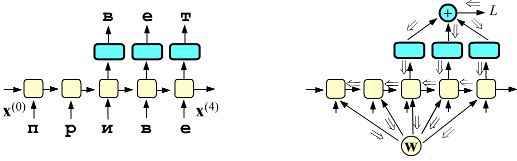
The errors are the logarithms of the probabilities (with the opposite sign) of the "correct" letters. From each of the three letters these errors are summed, giving the total loss $L$. During backpropagation, the gradient $g=1$ from $L$, having split, goes down, passing through the softmax function and the linear layer, and reaches the outputs of the last three cells. Then, passing through the cells, the gradients move left along the layer.
The set of parameters of the RNN cell in the right figure is denoted by the vector $\mathbf{w} = \{\mathbf{W},\mathbf{H},\mathbf{b},...\}$. Since all cells share the same parameters, the gradients from the cells arrive at $\mathbf{w}$ and are summed there.
Note that the total gradient entering the last (5th) cell is smaller than that entering the 4th and 3rd, because it does not receive the horizontal gradient.
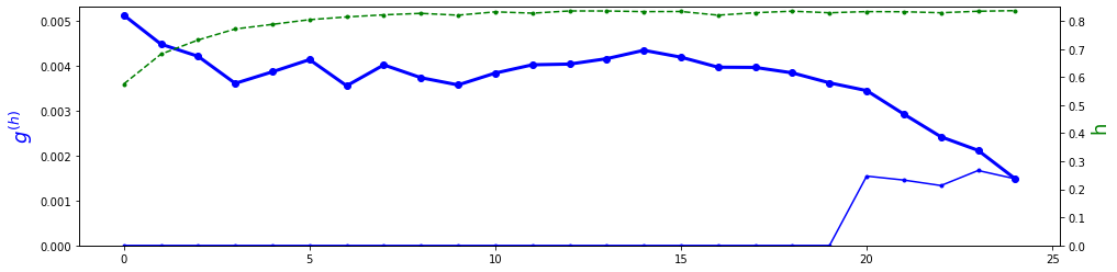
Below is a real example of the change in the length of the gradient (averaged over the batch) along the RNN layer. The layer has L=25 cells and the loss is computed on the last 5 outputs (E=10, H=50, one layer, GRU cells). The thick blue line is the total gradient entering the cell (from above and from the right); the thin line is the gradient entering only from above, and the dashed green line is the average length of the hidden state vector. The graph corresponds to the beginning of training:
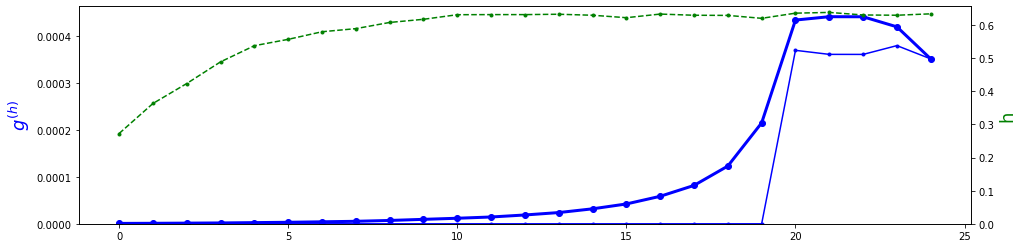
If you look at the graph from right to left, you can see that the gradient first starts to grow (vertical gradients are added to the "horizontal" ones). Then, when the injection of vertical gradients from the errors stops, the gradient monotonically fades toward the beginning of the sequence (vanishing gradient problem).
This situation is typical at the beginning of training (after the first epoch loss: trn=3.07 val=2.78). When the network is trained after 30 epochs loss: trn=1.12 val=1.10, the gradient fading may disappear (the average absolute value of the elements of the $H$ matrices, which are multiplied by the hidden state, increases from 0.12 to 0.42).
Gradients in cells
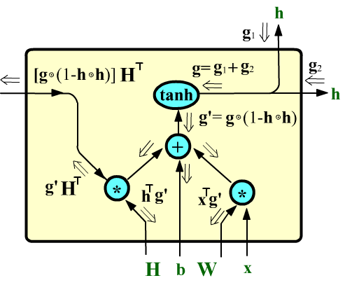 Suppose a gradient $\mathbf{g}$ enters a simple nn.RNN cell on the right along the hidden state line.
The derivative of the hyperbolic tangent $\tanh (x)$ is $1-\tanh^2(x)$.
At the output of the tanh node during the forward pass, the vector $\mathbf{h}$ was obtained.
Therefore, after passing through the $\tanh$ node, the gradient components are multiplied by
$1-\mathbf{h}\odot \mathbf{h}$, where the symbol $\odot$ means element-wise multiplication:
$(\mathbf{u}\odot\mathbf{v})_i = u_i v_i$.
Suppose a gradient $\mathbf{g}$ enters a simple nn.RNN cell on the right along the hidden state line.
The derivative of the hyperbolic tangent $\tanh (x)$ is $1-\tanh^2(x)$.
At the output of the tanh node during the forward pass, the vector $\mathbf{h}$ was obtained.
Therefore, after passing through the $\tanh$ node, the gradient components are multiplied by
$1-\mathbf{h}\odot \mathbf{h}$, where the symbol $\odot$ means element-wise multiplication:
$(\mathbf{u}\odot\mathbf{v})_i = u_i v_i$.
Taking into account the gradient transformation rules at the nodes of elementary operations, we obtain that at the cell output the gradient is $[\mathbf{g}\odot (1-\mathbf{h}\odot \mathbf{h})]\cdot \mathbf{H}^\top$. If $\mathbf{h}$ is close to $\pm 1$, the gradient decreases. Small components of the matrix $\mathbf{H}$ also reduce it.
After passing through n cells, the gradient entering the first cell will be multiplied by a factor of the form: $$ \mathbf{g}' = \bigr[\bigr[...\bigr[\mathbf{g}^{(n)} \odot (1-\mathbf{h}^{(n)}\odot \mathbf{h}^{(n)})\cdot \mathbf{H}^\top\bigr] \odot (1-\mathbf{h}^{(n-1)}\odot \mathbf{h}^{(n-1)})\cdot \mathbf{H}^\top\bigr]\,\odot ... \odot\, (1-\mathbf{h}^{(1)}\odot \mathbf{h}^{(1)})\bigr] \cdot \mathbf{H}^\top $$ Since the parameters of all cells are the same, the gradients entering them must be summed. The most significant gradients will be those from the last cells if the loss is computed only with respect to the last hidden state (i.e. the gradient from the loss enters only the last cell).
One possible strategy to combat fading is to start training by taking into account the errors of the outputs of all cells. Then, as the network becomes more trained, only the errors of the last cells are taken into account. You can also increase the variance of the initial random values of the matrix $\mathbf{H}$.
Recall that in a stack of fully connected layers, gradient fading leads to a complete stop of training. In a recurrent layer the fading problem is not as serious. Since all cells share the same parameters, they will still be updated due to the gradient in the last cells.
Additional reading :
- The Unreasonable Effectiveness of Recurrent Neural Networks
- Understanding LSTM Networks
- Building a LSTM by hand on PyTorch
- How to teach your neural network to generate poetry
