ML: Recurrent Networks in Keras
Introduction
Sometimes the training data is an ordered sequence. For example, time series (stock prices, sensor readings) or a sequence of natural language words. In such cases, it makes sense to use RNN (recurrent neural network).
As examples in Python, we will use the libraries numpy and keras:
import numpy as np                                # working with tensors

from keras.models import Sequential, Model
from keras.layers import SimpleRNN, LSTM, Dense, Embedding, Concatenate, Bidirectional
All examples can be found in the file: ML_RNN_Keras.ipynb. A discussion of RNN using the PyTorch framework can be found here.
SimpleRNN
A simple recurrent network consists of inputs connected cells with identical parameters. The network receives an ordered sequence of length inputs. Each element of the sequence is an f-dimensional vector $\mathbf{x}=\{x_0,...,x_{f-1}\}$ of features. The first vector is fed into the first cell, the second into the second, and so on. Each cell is characterized by a units-dimensional vector of hidden state: $\mathbf{h}=\{h_0,...,h_{u-1}\}$. This vector is the output of the cell (upward arrow), and the same vector is passed to the next cell. Inside the cell, the following computation is performed:

Since all cells are identical, the number of inputs does not affect the number of parameters. The matrix dimensions (shape) are: $\mathbf{W}:$(features, units), $~\mathbf{H}:$(units, units), $~\mathbf{b}:$( units, ), and the total number of parameters is:
params = (features + units + 1) * units
The initial hidden state vector $\mathbf{h}^{(-1)}$ (entering the first cell) is either equal to zero $\mathbf{0}$, or is taken to be the hidden state of the last cell from the previous sequence (or batch of sequences). Let’s examine the matrix multiplications in the hidden state computation in more detail.
Matrix multiplications
In an RNN cell, the input vector $\mathbf{x}^{(t)}$ and the hidden state vector of the previous cell $\mathbf{h}^{(t-1)}$ are combined (concatenated) and passed through a fully connected layer with the activation function than. The output of this layer becomes the hidden state of the current cell. Let's take a closer look at how the matrix computations work.
The feature vector $\mathbf{x}_t$ is multiplied by the weight matrix $\mathbf{W}$ on the left, as usual, so that batch rows can be added to it. For example, for input dimension features=3 and output dimension (hidden state size) units=2, we have:
$$ \begin{array}{|c|c|c|} \hline x^{(t)}_{0} & x^{(t)}_{1} & x^{(t)}_{2} \\ \hline \end{array} \cdot \begin{array}{|c|c|} \hline W_{00} & W_{01} \\ \hline W_{10} & W_{11} \\ \hline W_{20} & W_{21} \\ \hline \end{array} ~~ + ~~ \begin{array}{|c|c|} \hline h^{(t-1)}_{0} & h^{(t-1)}_{1} \\ \hline \end{array} \cdot \begin{array}{|c|c|} \hline H_{00} & H_{01} \\ \hline H_{10} & H_{11} \\ \hline \end{array} ~~+~~ \begin{array}{|c|c|} \hline b_{0} & b_{1} \\ \hline \end{array} ~~=~~ \begin{array}{|c|c|} \hline r^{(t)}_0 & r^{(t)}_1 \\ \hline \end{array} $$Such matrix multiplication can be made more compact by concatenating the vectors $\mathbf{x}^{(t)}$ and $\mathbf{h}^{(t-1)}$ and attaching the matrix $\mathbf{H}$ under the matrix $\mathbf{W}$:
$$ \begin{array}{|c|c|c|c|c|} \hline x^{(t)}_{0} & x^{(t)}_{1} & x^{(t)}_{2} & h^{(t-1)}_{0} & h^{(t-1)}_{1}\\ \hline \end{array} \cdot \begin{array}{|c|c|} \hline W_{00} & W_{01} \\ \hline W_{10} & W_{11} \\ \hline W_{20} & W_{21} \\ \hline H_{00} & H_{01} \\ \hline H_{10} & H_{11} \\ \hline \end{array} ~~+~~ \begin{array}{|c|c|} \hline b_{0} & b_{1} \\ \hline \end{array} ~~=~~ \begin{array}{|c|c|} \hline r^{(t)}_0 & r^{(t)}_1 \\ \hline \end{array} $$That's why the merged arrows of vectors $\mathbf{x}^{(t)},\mathbf{h}^{(t-1)}$ were drawn above. After computing the hyperbolic tangent of the multiplication result $\mathbf{r}^{(t)}$, we obtain the hidden state vector $\mathbf{h}^{(t)}= \tanh(\mathbf{r}^{(t)})$. If the multiplication is performed for all batch examples at once, then they are added as rows (below batch_size=3):
$$ \begin{array}{|c|c|c|c|c|} \hline x^{(t)}_{00} & x^{(t)}_{01} & x^{(t)}_{02} & h^{(t-1)}_{00} & h^{(t-1)}_{01}\\ \hline x^{(t)}_{10} & x^{(t)}_{11} & x^{(t)}_{12} & h^{(t-1)}_{10} & h^{(t-1)}_{11}\\ \hline x^{(t)}_{20} & x^{(t)}_{21} & x^{(t)}_{22} & h^{(t-1)}_{20} & h^{(t-1)}_{21}\\ \hline \end{array} \cdot \begin{array}{|c|c|} \hline W_{00} & W_{01} \\ \hline W_{10} & W_{11} \\ \hline W_{20} & W_{21} \\ \hline H_{00} & H_{01} \\ \hline H_{10} & H_{11} \\ \hline \end{array} ~~+~~ \begin{array}{|c|c|} \hline b_{0} & b_{1} \\ \hline \end{array} ~~=~~ \begin{array}{|c|c|} \hline r^{(t)}_{00} & r^{(t)}_{01} \\ \hline r^{(t)}_{10} & r^{(t)}_{11} \\ \hline r^{(t)}_{20} & r^{(t)}_{21} \\ \hline \end{array} $$In this case, the bias row $(b_1~b_2)$ of shape (1,2) is added to each row of the matrix of shape (3,2) according to the broadcasting rule used in numpy.
SimpleRNN in Keras
When creating a recurrent layer, it is necessary to specify the dimension of the hidden state units and (if it is the first layer) the dimensions of the input vectors features (a non-first layer will obtain these parameters from the previous layers):
units    = 4          # hidden state dimension   = dim(h)
features = 2          # input vector dimension   = dim(x)
inputs   = 3          # number of inputs (RNN cells)

model = Sequential()
model.add(SimpleRNN(units=units, input_shape=(inputs, features))) # Output Shape: (None, 4)
By default, this layer returns only the hidden state of the last cell in the layer (see the next section). Therefore, the tensor returned by the layer has the shape (None, units) and does not depend on the number of cells (inputs) or their dimensionality (features). None corresponds to an arbitrary number of examples in the batch.
Since all cells are identical, the number of inputs can be omitted by setting None:
model = Sequential()
model.add(SimpleRNN(units=units, input_shape=(None, features)))   # Output Shape: (None, 4)
In this case, the same model can process not only different batches, but also batches with input sequences of different lengths (but all examples in the same batch must have the same sequence length):
model.predict( np.zeros( (2, 3, features)  ))
model.predict( np.zeros( (2, 4, features)  ))
In the first predict the batch consists of two “samples” with three inputs each. In the second, the samples in the batch have four inputs.
Sometimes, when defining a model, it is necessary to strictly specify the batch size. Then, as usual, use batch_input_shape instead of input_shape:
model = Sequential()
model.add(SimpleRNN(units=units, batch_input_shape=(10, inputs, features)))  #    (10, 4)
Many-to-one or Many-to-many
A recurrent layer can return either the hidden state of only the last cell (return_sequences = False) or the hidden states of all cells in the layer (return_sequences = True):
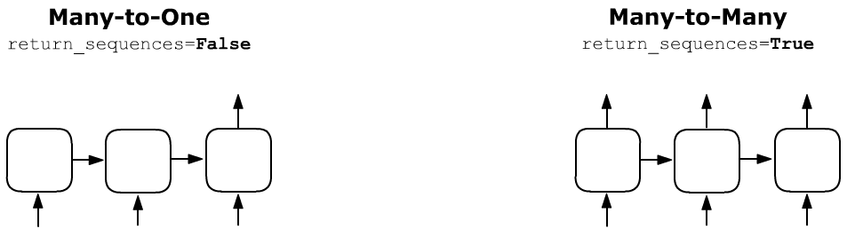
Depending on the mode, the output shape of the recurrent layer changes. If return_sequences = True (all cells return), then the output shape of the layer is (batch_size, inputs, units):
model = Sequential()
model.add(SimpleRNN(units=4, input_shape=(None,2), return_sequences = True ))

Output Shape: (None, None, 4)
With return_sequences = False (the default in Keras), the output shape of the layer is (batch_size, units):
model = Sequential()
model.add(SimpleRNN(units=4, input_shape=(None, 2), return_sequences = False ))

Output Shape:  (None, 4)
The number of parameters in the layer (28 in this example) does not depend on the value of return_sequences (it is the number of elements in the cell’s matrices).
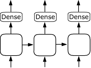 If after a recurrent layer with return_sequences = True there is, for example,
a fully connected Dense layer, then it is applied with the same set of parameters
to the output of each cell:
If after a recurrent layer with return_sequences = True there is, for example,
a fully connected Dense layer, then it is applied with the same set of parameters
to the output of each cell:
model = Sequential()
model.add(SimpleRNN(units=4, input_shape=(None,2), return_sequences=True))
model.add(Dense(units=8))

Output Shape: (None, None, 8)
Similarly, instead of a Dense layer, you can use other recurrent layers, stacking them to build deep learning architectures.
A few more parameters
When defining a recurrent layer, the following parameters are also available:
- activation="linear" - linear activation function for the cell (instead of "tanh" by default). Any available activation functions can be used. The values of the tanh function lie in the range [-1...1]. This is usually preferable to [0...1] ("sigmoid") or [0...infty] ("relu"). When the hidden state passes through the layer, it is multiplied by the same matrix in each cell. Therefore, if the components of vector $\mathbf{h}$ are always positive, the hidden state risks becoming very large or collapsing to zero.
- stateful = True - do not reset the hidden state $\mathbf{h}^{(-1)}$ to zero after each batch, but instead set it equal to the last cell's state from the previous iteration (see the example below).
A toy example
Let's consider the linear model $h_t = x_t+ h_{t-1}$ (all “vectors” here are single-component, so time indices are written below). As inputs $x_t$ we will use two batches with one sample each: $\{1,2,3\}$ and $\{4,5,6\}$. If we work in the mode stateful = False, then before each batch $h_{-1}=0$. When stateful = True, for the first batch $h_{-1}=0$, and for the second $h_{-1}$ is equal to the last hidden state:
Let's perform these computations using a recurrent network:
model = Sequential()
model.add(SimpleRNN(units=1, batch_input_shape=(1, 3, 1),
                    activation="linear", stateful = True, name='rnn') )
Since by default return_sequences=False, the network will return
only the hidden state of the last cell (the bold numbers in the example above).
Let’s set the values of the recurrent cell "matrices". In our example, $\mathbf{W}$ and $\mathbf{H}$ each consist of a single element and have shape (1,1). The bias $\mathbf{b}$ is equal to zero. The layer parameters are packed in a list in the order [ W, H, b ]:
W, H, b  = np.array([[1]]), np.array([[1]]), np.array([0])
model.get_layer('rnn').set_weights(([ W, H, b ]))              # change weights
Now we can perform the computations:
res = model.predict(np.array([ [ [1], [2], [3] ]  ] ))
print("res:",np.reshape(res, -1) )                             # res: [6.]

res = model.predict(np.array([ [ [4], [5], [6] ]  ] ))
print("res:",np.reshape(res, -1) )                             # res: [21.]
If we set stateful = False, then the results would be 6
and 15.
LSTM
Standard RNNs handle "long-term dependencies" poorly and mostly capture correlations between neighboring elements of a sequence. Recurrent layers with LSTM cells handle long-term dependencies much better.
In addition to the hidden state $\mathbf{h}$ passed from one cell to the next, an LSTM layer also passes a memory state $\mathbf{c}$. This vector has dimension units, just like the usual hidden state $\mathbf{h}$. The vectors $\mathbf{c}$ regulate which features should be forgotten and which should be remembered when passed to the next cell. Through this mechanism, long-term memory is implemented.
Inside an LSTM cell, instead of a single neural-network layer (as in SimpleRNN), there are four layers. The sigmoid layers $\sigma$ produce output vectors with values in $[0...1]$, and the hyperbolic tangent $\tanh$ produces values in $[-1...1]$.
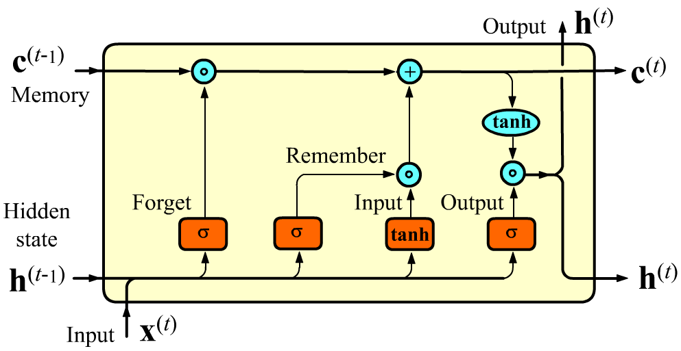
The hidden state $\mathbf{h}$ is computed similarly to SimpleRNN (but using a sigmoid instead of $\tanh$, see the last rectangle). After that, it is multiplied by $\tanh(\mathbf{c})$. The hyperbolic tangent is applied independently to each component of the vector $\mathbf{c}$, making the corresponding component of $\mathbf{h}$ positive or negative (or possibly zero if that feature component is not important going forward).
Before this computation, the value of the memory vector $\mathbf{c}^{(t-1)}$ is updated. First, $\mathbf{x}^{(t)} and \mathbf{h}^{(t-1)}$ pass into a fully connected layer with a sigmoid [0...1] at the output. This is called the forget gate. The output dimension of this layer equals units (the dimension of $\mathbf{h}$ and $\mathbf{c}$). The components of this output vector are multiplied by the components of the previous memory vector $\mathbf{c}^{(t-1)}$ (without convolution!). Through this multiplication some features in $\mathbf{c}^{(t-1)}$ are forgotten (if multiplied by 0), and some are preserved (if multiplied by 1). An example of a case where forgetting is needed: "She put on a red hat and a green skirt" ("green" after a noun may forget "red")
The next two gates work similarly, implementing memorization. The features that need to be remembered are added to the vector $\mathbf{c}$. The $\tanh$ layer forms "candidate features," scaling them to the interval [-1...1]. The sigmoid [0...1] layer strengthens or weakens the importance of the feature to be memorized.
More specifically, computations in an LSTM cell look as follows: $$ \left\{ \begin{array}{lclclcl} \mathbf{F} &=& ~~~~~~\sigma(\mathbf{x}^{(t)}\, \mathbf{W}_{f} &+& \mathbf{h}^{(t-1)}\, \mathbf{H}_{f} &+& \mathbf{b}_f),\\ \mathbf{I} &=& ~~~~~~\sigma(\mathbf{x}^{(t)}\, \mathbf{W}_{i} &+& \mathbf{h}^{(t-1)}\, \mathbf{H}_{i} &+& \mathbf{b}_i),\\ \mathbf{R} &=& \text{tanh}(\mathbf{x}^{(t)} \mathbf{W}_{r} &+& \mathbf{h}^{(t-1)}\, \mathbf{H}_{r} &+& \mathbf{b}_r),\\ \mathbf{O} &=& ~~~~~~\sigma(\mathbf{x}^{(t)}\, \mathbf{W}_{o} &+& \mathbf{h}^{(t-1)}\, \mathbf{H}_{o} &+& \mathbf{b}_o), \end{array} \right. ~~~~~~~~~~~~~~~~~~ \left\{ \begin{array}{lcl} \mathbf{c}^{(t)} &=& \mathbf{F} * \mathbf{c}^{(t-1)} + \mathbf{I} * \mathbf{R},\\[2mm] \mathbf{h}^{(t)} &=& \tanh\bigr(\mathbf{c}^{(t)}\bigr) * \mathbf{O}. \end{array} \right. $$
The dimensions of the matrices are [feature$=\dim(\mathbf{x}),~~~~$ units$=\dim(\mathbf{h}),~\dim(\mathbf{c})$]: $$ \begin{array}{llllll} \mathbf{W}_{i}, &\mathbf{W}_{f}, &\mathbf{W}_{r}, &\mathbf{W}_{o}: &\mathrm{(features, units)},\\ \mathbf{H}_{i}, &\mathbf{H}_{f}, &\mathbf{H}_{r}, &\mathbf{H}_{o}: &\mathrm{(units, units)},\\ \mathbf{b}_i, &\mathbf{b}_f, &\mathbf{b}_r, &\mathbf{b}_o: &\mathrm{(1, units)}. \end{array} $$Bidirectional layer
 Sometimes in sequences there is an influence on the present not only from the past,
but also from the future. For example, the meaning of a given word in a sentence is determined by the whole sentence,
and not only by the words that precede it.
Sometimes in sequences there is an influence on the present not only from the past,
but also from the future. For example, the meaning of a given word in a sentence is determined by the whole sentence,
and not only by the words that precede it.
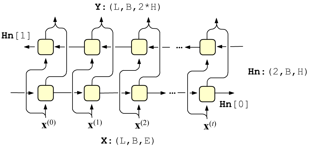
In this case it is appropriate to use two recurrent layers together, in the first of which the hidden states propagate from left to right, and in the next layer - from right to left. The input vectors are fed independently to each layer, and their outputs are concatenated. The cell weights of each layer are different.
If return_sequences = False, then, as before, the output of the Bidirectional layer receives only the concatenation of the outputs of the last cells of each layer.
VOC_SIZE, VEC_DIM, inputs = 100, 8, 3

model = Sequential()
model.add(Embedding(input_dim=VOC_SIZE, output_dim=VEC_DIM, input_length=inputs))

model.add(Bidirectional(SimpleRNN(units=4, return_sequences=True)))      # (None,3,8)

model.add(Dense(units = 1, activation='sigmoid'))                        # (None,3,1)
Above, the first layer is Embedding which receives the vocabulary size VOC_SIZE and the dimension of the vector space VEC_DIM and creates a 2-dimensional array (VOC_SIZE, VEC_DIM). Embedding converts an integer at the input (a word index) into a vector that corresponds to this word at the output. In Embedding you can specify the number of inputs input_length, and then it, as well as the number of examples in a batch (batch_size), is considered undefined (the network can process any number of inputs).
Three vectors (inputs=3) of dimension VEC_DIM=8 are fed to the 3 inputs of the Bidirectional layer. Since the dimension of the hidden state is units=4, each cell receives an 8-dimensional vector (concatenation 4+4=8).
The return_state parameter
When defining a network functionally, it is possible to return not only the outputs of the cells, but also all hidden states of the last cell.
units    = 4                   # dimension of the hidden state   = dim(h)
features = 2                   # dimension of the inputs         = dim(x)
inputs   = 3                   # number of inputs (RNN layer cells)

inp    = Input( shape=(inputs, features) )
rnn    = LSTM (units, return_sequences=True, return_state=True)(inp)

model  = Model(inp, rnn)       #   [(None, 3, 4), (None, 4), (None, 4)]
The list of matrices corresponds to all outputs (return_sequences=True), the hidden state h and the hidden memory state c.
inp    = Input(shape=(inputs, features) )
rnn    = LSTM (units, return_sequences = True, return_state=True)

_,h,s  = rnn(inp)              # ignore the outputs (the first matrix)

con    = Concatenate()([h,s])  # (None, 8)

model  = Model(inp, con)
In the case of a bidirectional layer
inp    = Input(shape=(inputs, features) )
rnn    = LSTM (units, return_sequences = True, return_state=True)
bid    = Bidirectional(rnn)(inp)

Output shape: [(None, 3, 8), (None, 4), (None, 4), (None, 4), (None, 4)]
