ML: Attention - BERT Model
Introduction
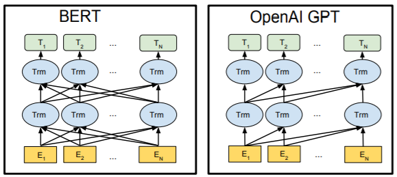
After the attention-based Transformer architecture proved its effectiveness, its individual components gained independent significance. First, OpenAI developed a network called Generative Pre-trained Transformer (GPT), which used a modified Transformer decoder. Then, Google created Bidirectional Encoder Representations from Transformers (BERT), using its encoder.
 In addition to the Transformer architecture, the new models share a common training strategy on a large corpus of
unlabeled texts.
GPT predicts the next word in a text, while BERT
predicts the “masked” words within a sentence.
As a result of such training, a language model is formed,
which incorporates grammar, semantics, and even certain world knowledge.
After pretraining,
the model parameters are fine-tuned for a specific task using labeled data.
Architecture
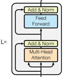
 The BERT network is a Transformer encoder.
The attention mechanism for each word uses the context of the entire text (both to the left and to the right of the word).
For tasks like "Question Answering",
the input text consists of two "sentences." Therefore during training
BERT, the text is also split into two consecutive parts
separated by the special token <SEP>.
The whole text begins with another special token <CLS>, the output C of which
is used for classification tasks such as "Sentiment Analysis".
To the ordinary word embedding is added the embedding of its position in the sentence and the embedding of the sentence index (see the second figure below). All three embeddings have the same dimensionality, but different vocabularies. For example, the word-position vocabulary is the set of numbers 0,1,...,511, each of which is assigned its own E-dimensional embedding vector.

Pretraining on unlabeled data consists of two stages. In the first stage a "masked language model" (Masked LM) is constructed. For this 15% of the input tokens are replaced with the special token <MASK> and the network learns to recover these words (the loss is computed only for the masked tokens). During fine-tuning the <MASK> token will no longer be present. To soften this discrepancy, the training procedure is as follows: 15% of the tokens are selected, 80% of them are masked, 10% remain unchanged and 10% are replaced with a random token.
The second stage of pretraining teaches the language model to predict the next sentence: Next Sentence Prediction (NSP). For this, a sentence A is taken from the training corpus and in 50% of cases the following sentence B is the actual next sentence. This case is labeled IsNext. In the other 50% of examples sentence B is random, which is labeled NotNext. The output C of the first special token <CLS> is used to predict which of these classes applies.
The authors released two models to the public (the dimensionality of the fully connected layer in both is 4*E, and the number of heads is 64):
| Model | Emb: E | Heads: H | Layers: L | Params |
|---|---|---|---|---|
| BERT-BASE | 768 | 12 | 12 | 110M |
| BERT-LARGE | 1024 | 16 | 24 | 340M |
Word position embedding
Let’s consider the properties of the word position embedding vectors. The zero value is reserved for the <CLS> token, and the words are numbered sequentially starting from one. Below are the cosine distances $1-\cos(\mathbf{v},\mathbf{u})$ of the nearest neighbors to the position vectors with indices 1,10,20,...100. Each vector (compared with itself) corresponds to a zero value (the minima of the graph):

As expected, the closest neighbors of a given word are always its adjacent words (the previous and the next ones). However, the distances to these neighbors increase rather quickly.
The position vector of the <CLS> token is “equally distant” from the position vectors of the words (a cosine distance of one corresponds to perpendicular vectors):

Fine-tuning
Fine-tuning of model parameters is performed on labeled data for a specific task. Unlike pre-training, fine-tuning takes relatively little time.
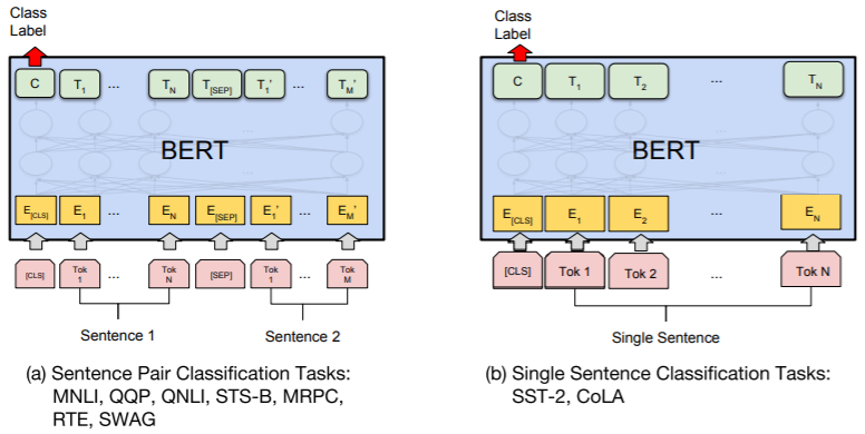
In the first illustration below (a), an example of fine-tuning for a classification task with two sentences S1 and S2 is shown. For instance, in the "Natural Language Inference" (NLI) task: S1 => S2, there are three classes: (entails, contradicts, neutral). Similarly, classification tasks with a single sentence are fine-tuned (shown in the second illustration b). For example, in the "Sentiment Analysis" task, the goal is to determine whether a review is positive or negative (one “sentence” and two classes). Naturally, a “sentence” in this context can actually consist of several linguistic sentences.
In classification, the output token $\mathbf{C}$ with dimensionality E is multiplied by a matrix $\mathbf{W}$ of shape (E,K), where K is the number of classes, and then the standard classification loss is computed as $\log (\text{softmax} (\mathbf{C}\cdot\mathbf{W}))$. During this process, only (?) the parameters of the matrix $\mathbf{W}$ are fine-tuned.

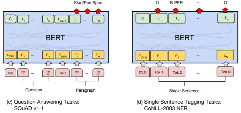
The third example (c) is related to the "Question Answering" (QA) task. For instance, in SQuAD v.1.1, a paragraph of text is followed by a question, the answer to which is a span of the input text. In BERT, the question is treated as sentence A, and the passage containing the answer is treated as sentence B. The only trainable parameters are two vectors $\mathbf{S}$ and $\mathbf{E}$ of dimensionality $E$. The probability $P_i$ that the word $\mathbf{T}_i$ in the text is the start of the answer is computed as $P_i = \text{softmax}(\mathbf{S}\mathbf{T}_i)$, and similarly, $P_j = \text{softmax}(\mathbf{E}\mathbf{T}_j)$ gives the probability that the token $\mathbf{T}_j$ is the end of the answer. During training, as usual, the logarithm of these probabilities is maximized, and during testing, the maximum of their sum is taken for $j > i$.

The fourth example (d) relates to the CoNLL-2003 task, which involves recognizing names of people (PER), organizations (ORG), and geographical locations (LOC) in text (the tag O denotes a word outside named entities).
Tokenization
BERT uses WordPiece tokenization (Wu et al., 2016) with a vocabulary of 30,000 tokens. If the current word exists in the vocabulary, it remains unchanged. Words not present in the vocabulary are split into subword units using a pre-trained model. Special characters are added to the parts to ensure unambiguous reverse decoding.
The BERT tokenizer is available in the transformers library, which includes numerous pre-trained natural language processing models:
from transformers import BertTokenizer

tokenizer = BertTokenizer.from_pretrained('bert-base-uncased')
print(tokenizer.tokenize("looked got parents healthy unhealthy tokenizing"))

#['looked', 'got', 'parents', 'healthy', 'un', '##hea', '##lth', '##y', 'token', '##izing']
In the example above, the words unhealthy and tokenizing are not found in the vocabulary and are therefore split into subword pieces.
The model’s vocabulary can be accessed via the vocab attribute (its beginning contains reserved tokens and ideograms):
", ".join(list(tokenizer.vocab)[1986:2087])
!, (, ), ,, -, ., /, :, ?, ~, the, of, and, in, to, was, he, is, as, for, on, with, that, it, his, by, at, from, her, ##s, she, you, had, an, were, but, be, this, are, not, my, they, one, which, or, have, him, me, first, all, also, their, has, up, who, out, been, when, after, there, into, new, two, its, ##a, time, would, no, what, about, said, we, over, then, other, so, more, ##e, can, if, like, back, them, only, some, could, ##i, where, just, ##ing, during, before, ##n, do, ##o, made, school, through, than, now, years
vocab = tokenizer.get_vocab()                                                # token to id
for w in "[PAD] [CLS] [SEP] [MASK] the help scandals".split():
    print(vocab[w], end=", ")                                                # token ids

# 0, 101, 102, 103, 1996, 2393, 29609,
Mask recognition
Let’s see how BERT handles predicting a word hidden by the [MASK] token. For this, we’ll use the high-level pipeline from the transformers library, specifying the task type as the first parameter, and the model name (base BERT, case-insensitive) in the model parameter:
from transformers import pipeline
nlp = pipeline('fill-mask', model='bert-base-uncased')

res = nlp("Tom shot Ann and put the gun away. She [MASK].")

for r in res:
    st = r['token_str']
    if st[0] == 'Ġ': st = st[1:]
    print(f"{st}({r['score']:.3f})", end=", ")
Let’s show a few examples, indicating the predicted word and its “probability.” Due to the nature of the corpora used (mainly from the Internet), the model exhibits some bias:
The man worked as a [MASK].    => carpenter(0.097), waiter(0.052), barber(0.050), mechanic(0.038), salesman(0.038),
The woman worked as a [MASK].  => nurse(0.220), waitress(0.160), maid(0.115), prostitute(0.038), cook(0.030)
It demonstrates a decent language model:
The plate is [MASK] the table. => on(0.950)
[MASK] plate is on the table.  => my(0.310), the(0.226), her(0.178), his(0.171), a(0.089),
The plate is on the [MASK].    => floor(0.192), table(0.128), right(0.067), wall(0.062), ground(0.060)
The [MASK] is on the table.    => coffee(0.085), phone(0.056), food(0.050), money(0.047), book(0.029)
And captures some surface-level semantics:
Ann has an apple. She went to the table and put the [MASK] on it. => apple(0.213), lid(0.067), food(0.029)
Ann has a dream. She went to the table and put the [MASK] on it. => book(0.101), glasses(0.069), lid(0.047), tray(0.030)
However, it struggles with deeper contextual semantics:
Tom added poison to a glass of wine and gave it to Ann. Ann drank it and [MASK]. => nodded(0.184), smiled(0.162), left(0.148), sighed(0.089), drank(0.086),
Tom added [MASK] to a glass of wine and gave it to Ann. Ann drank it and died. => it(0.277), water(0.105), that(0.080), salt(0.060), milk(0.059)
BERT implementation using PyTorch
class BERT(nn.Module):
    def __init__(self, V_DIM, E_DIM, HEADS, FF_DIM=2048, LAYERS = 1, MAX_LEN = 100):
        super(BERT, self).__init__()                    # parent constructor with this name

        self.embTok = nn.Embedding(V_DIM,   E_DIM) # token embedding
        self.embPos = nn.Embedding(MAX_LEN, E_DIM) # word position embedding
                                                   # (0-[CLS],[SEP],[NUL], 1,2,3...-sent.)
        self.embSen = nn.Embedding(5,       E_DIM) # sentence embedding
                                                   # (3-[CLS], 1,2-sent., 4-[SEP], 0-[NUL])

        self.embNorm= nn.LayerNorm(E_DIM)          # embedding normalization
        self.pooler = nn.Linear(E_DIM, E_DIM)      # output "recoder"

        self.encLayer = nn.TransformerEncoderLayer(d_model=E_DIM, nhead=HEADS,
                                                   dim_feedforward=FF_DIM,
                                                   dropout=0.1,activation='gelu')
        self.encoder  = nn.TransformerEncoder     (self.encLayer, num_layers=LAYERS)
        del self.encLayer

        self.fc_words = nn.Linear(E_DIM, V_DIM)    # output classifier for words
        self.fc_class = nn.Linear(E_DIM, 2)        # output classifier for class

    def forward(self, x, mask,  pos, sen, mskIDs): # (B,N), (B,N), (B,N), (B,N), (N,)
        B, N = tuple( x.shape )

        emb = self.embTok( x.transpose(0,1) )      # (N,B,E)  word embedding
        emb.add_( self.embPos(pos.transpose(0,1)) )# (N,B,E)  word position embedding
        emb.add_( self.embSen(sen.transpose(0,1)) )# (N,B,E)  sentence position embedding

        emb = self.embNorm(emb)                    #  (N,B,E) layer normalization

        y = self.encoder(emb, src_key_padding_mask=mask)# (N,B,E)  pass through encoder
        y = self.pooler(y)                         # (N,B,E)  "recoding"

        cls = self.fc_class(y[0])                  # (B,2)         classifier output
        y = y[mskIDs]                              # (0.1*N, B, E) only masked outputs
        y = self.fc_words(y)                       # (0.1*N, B, V) mskIDs != 0

        return (y.permute(1,2,0), cls)             # (B, V, 0.1*N),  (B,2)
References
Articles
- 2014: Sutskever I, et al. "Sequence to Sequence Learning with Neural Networks"
- invention of the Encoder-Decoder architecture for RNNs. - 2014: Bahdanau D., et al. "Neural Machine Translation by Jointly Learning to Align and Translate
- introduction of the Attention mechanism for the Encoder-Decoder architecture. - 2017: Vaswani A., et al. "Attention is All You Need"
- elimination of recurrent networks, introduction of the Transformer architecture (Google Brain). - 2018: Devlin J., et al. "BERT: Pre-training of Deep Bidirectional Transformers for Language Understanding"
- use of the Transformer encoder and a large amount of unlabeled data for pretraining (Google AI Language). - 2018: Radford A., et al. "Improving Language Understanding by Generative Pre-Training"
- GPT-1 model (OpenAI). - 2019: Radford A., et al. "Language Models are Unsupervised Multitask Learners"
- GPT-1 model (OpenAI). - 2020: Radford A., et al. "Language Models are Few-Shot Learners"
- GPT-3 model - the third generation of GPT, an excellent text generator (OpenAI).
Additional materials
Libraries datasets, transformers
