ML: Transformer
Introduction
In this document we continue to discuss the attention mechanism. Multi-head attention was introduced in the paper "Attention is All You Need" (2017) for the Transformer architecture. This was a variant of the encoder-decoder for the translation task that did not use recurrent layers. Instead, sequences of word vectors were passed through several layers with masked attention. As a result, parallelization became possible, which significantly accelerated training (compared to recurrent networks).
Later, various parts of the transformer were used in such models as GPT (2018) and BERT (2018), which are covered in the next document.
General Architecture
From the point of view of structure and training methods, the transformer looks similar to an encoder-decoder based on recurrent networks. The encoder receives a sequence of words in the source language as input. The vectors of these words, after passing through a sequence of self-attention layers, change taking into account the context of the entire sentence. In the figure below they are denoted as memory ("memory of the source sentence"):
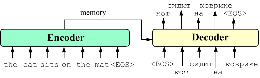
The decoder in teacher forcing mode receives this memory and the words of the translation sentence as input. At the output, it learns to predict the same translation shifted left by one word. In test mode (or "honest" training), the decoder is first fed the service word "<BOS>" (begin of sentence) and is expected to output the word "cat" at the output. Then "<BOS> cat" is fed as input, and "cat sits" is received at the output, and so on, until the decoder outputs "<EOS>" (end of sentence).
The encoder and decoder consist of a stack of identical blocks that perform "deep" transformation of the input tensors.
Transformer Encoder
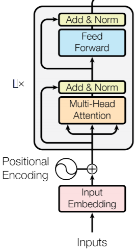
Let us consider the transformer encoder in more detail (figure on the right). A tensor of shape (N,B,E) is fed to its input, where N is the number of words in the input sequence, B is the number of simultaneously processed examples (batch), and E is the dimension of their embedding vectors. This tensor is passed through the multi-head self-attention function (Multi-Head Attention): the three arrows in the figure - these are matching queries, keys, and values. The result is added to the original tensor and normalized (see below). The resulting tensor is fed to a fully connected layer (Feed Forward) with two linear transformations (after the first - the activation function ReLU): $$ \text{FFN}(\mathbf{x}) = \max(0,~\mathbf{x}\cdot\mathbf{W}_1+\mathbf{b}_1)\cdot\mathbf{W}_2+\mathbf{b}_2. $$ The output of this layer is again summed with its input and normalized. Such computations are repeated several times (the multiplier L× in the figure means L such layer-blocks with different parameters). At the output of the last block, a tensor of the original shape (N,B,E) is obtained, which describes the words of the sequence taking into account the context of the entire text.
☝ Adding the input and output of the layer is a common practice in deep learning. Thanks to this, the gradient during backpropagation more easily reaches the beginning of the stack of layers. Indeed, in the addition node gradient copying occurs. One version passes through the layer and fades on nonlinear activation functions. The second bypasses the layer without change and amplifies its faded (and changed) copy.
☝ Normalization combats the situation when the weights of a neuron "drive" its output to very large or very small values, which slows down the training process. To eliminate this effect, the mean value is subtracted from the neuron outputs (before or after the activation function) and the result is divided by the standard deviation (square root of the variance). There are two methods for normalizing hidden layer neurons: batch (2015) and layer (2016) normalization. In the first method, averaging is performed over batch examples, and in the second - over all neurons of a given layer. Both methods accelerate training, but the second is simpler, because it works the same way during training and testing and does not depend on batch size. In the Transformer, averaging is performed over all components of the embedding vector independently for each input (word).
Encoder in PyTorch
In PyTorch the transformer encoder is built in two stages. First, TransformerEncoderLayer is defined, and then with its help the actual encoder TransformerEncoder is created:
✒ nn.TransformerEncoderLayer(d_model, nhead, dim_feedforward=2048, dropout=0.1,activation='relu')
Parameters: d_model = E – input dimension (vector of one token), nhead = H – number of heads (must be a divisor of the d_model parameter), dim_feedforward – dimension of the fully connected network. The activation function activation is used in the fully connected layer Feed Forward, and dropout sets the fraction of matrix elements that are randomly set to zero (fight against overfitting at the training stage). The dropout layer is placed immediately after the softmax function in nn.MultiheadAttention.
✒ nn.TransformerEncoder(encoder_layer, num_layers, norm=None)
The parameter encoder_layer is an instance of the TransformerEncoderLayer class, and num_layers = L sets the number of sequential blocks similar to the one shown in the figure above.
Here is an example of creating a transformer encoder:N, B, E, H = 10, 32, 512, 8 # number of words, batch size, embedding dimension, heads encoder_layer = nn.TransformerEncoderLayer(d_model=E, nhead=H) transformer_encoder = nn.TransformerEncoder (encoder_layer, num_layers=1) src = torch.rand(N, B, E) out = transformer_encoder(src) # out.shape == src.shapeThe list of parameters for one layer looks like this (the prefix layers.0. is omitted in the names):
self_attn.in_proj_weight  : 786432  (1536, 512)  # (3*E, E)  Wq, Wk, Wv
self_attn.in_proj_bias    :   1536  (1536,)      # (3*E,)    Bq, Bk, Bv
self_attn.out_proj.weight : 262144  (512, 512)   # (E,E)     Wo
self_attn.out_proj.bias   :    512  (512,)       # (E,)      Bo

linear1.weight            :1048576  (2048, 512)  # (dim_feedforward, E)  W1
linear1.bias              :   2048  (2048,)      # (dim_feedforward,)    B1
norm1.weight              :    512  (512,)       # (E,)
norm1.bias                :    512  (512,)       # (E,)

linear2.weight            :1048576  (512, 2048)  # (E, dim_feedforward)  W2
linear2.bias              :    512  (512,)       # (E,)                  B2
norm2.weight              :    512  (512,)       # (E,)
norm2.bias                :    512  (512,)       # (E,)

total                     :3152384
PyTorch stores linear transformation matrices in transposed form: $\text{line}(\mathbf{x})=\mathbf{x}\cdot \mathbf{W}^T+\mathbf{b}$. Therefore, in the fully connected layer multiplications occur: (*,E) @ (E, FF) @ (FF, E) = (*,E), where FF = dim_feedforward.
In Vaswani A., et al., (2017), as above, the values E = 512, FF = 2048 were used, so in the Feed Forward module the embedding vector dimensions are first increased by 4 times, and then returned to the original value.
Word Position Encoding
Unlike recurrent networks, the transformer architecture does not directly use information about the sequence of words. The situation can be fixed by mixing into the embedding of each word the "number" of its position in the sequence (positional embedding). There are several ways to encode the position of a word.
In the original paper (2017) quite specific periodic functions of the following form were chosen: $$ \text{PosEmb}(\text{pos},~2i) = \sin(\text{pos}/10000^{2i/E}),~~~~~~~ \text{PosEmb}(\text{pos},~2i+1) = \cos(\text{pos}/10000^{2i/E}), $$ where pos is the word number in the sentence, and $i$ is the component number of the embedding vector. The resulting $E$-dimensional embedding vectors were added to the word embedding vectors.
Later (GPT, BERT) trainable position encoding vectors were used. For this, in addition to the embedding of the vocabulary words, a separate (also $E$-dimensional) positional embedding is introduced (for each position pos of the word in the sentence its own vector). The word and position vectors, as above, are added and then fed into the transformer encoding.
Decoder
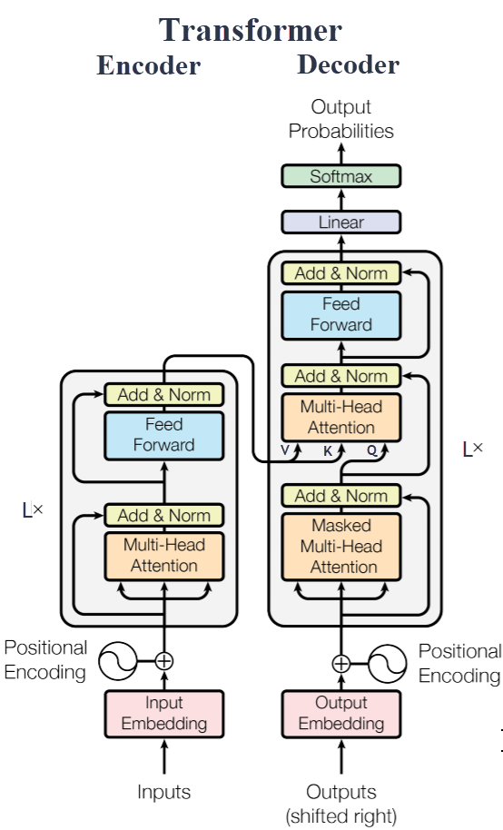 Now let us add a decoder to the encoder, obtaining the full Transformer architecture.
The decoder receives the words of the target translation sentence as input.
These words are vectorized (with an embedding different from the encoder) and position number vectors are added to them
(positional encoding).
Now let us add a decoder to the encoder, obtaining the full Transformer architecture.
The decoder receives the words of the target translation sentence as input.
These words are vectorized (with an embedding different from the encoder) and position number vectors are added to them
(positional encoding).
Then the vectors pass through a self-attention block (as in the encoder) to clarify the contextual meaning of the vectors. Unlike the encoder, this is self-attention with a mask (Masked Multi-Head Attention), so that the decoder does not look into the "answer" (see below for details). The output of the self-attention block is summed with its input and normalized.
After that, the attention mechanism on the words of the source language sentence is turned on (after their processing by the encoder). In this case, the queries are the decoder words, and the encoder vectors act as keys and values (see letters Q,K,V in the picture). The output is again summed with the input and normalized.
The decoder block is completed by a fully connected network (Feed Forward) of two layers (as in the encoder). The decoder has several such sequential blocks (their number L× usually coincides with the number of encoder blocks). Naturally, the training parameters for the blocks differ.
At the output of the stack of identical blocks there is a fully connected layer Line with the number of neurons equal to the size of the vocabulary. Its outputs are normalized by the softmax layer, giving the probability of each translation word.
Transformer in PyTorch
The transformer can be assembled from the encoder and decoder (for which there is its own class nn.TransformerDecoder, similar to nn.TransformerEncoder). However, you can immediately use the nn.Transformer class:
✒ nn.Transformer
(d_model=512, nhead=8, num_encoder_layers=6, num_decoder_layers=6, dim_feedforward=2048, dropout=0.1, activation='relu',
custom_encoder=None, custom_decoder=None)
✒ nn.Transformer.forward
(src, tgt, src_mask=None, tgt_mask=None, memory_mask=None, src_key_padding_mask=None,
tgt_key_padding_mask=None, memory_key_padding_mask=None)
Masks
For convenience of working with sequences of variable length (when forming batches), the hyperparameters $N$ and $M$ are set to be sufficiently large and shorter sentences are "padded" with a special token <PAD> with a dedicated index (usually 0). For example, let $B, N=1, 10$ (one example and a maximum of ten words in the source sentence). Then for the example from the beginning of the document, the sequence fed to the encoder looks like this:
The cat sits on the mat . <PAD> <PAD> <PAD>Since the words <PAD> must be ignored, not only the tensor $(N,B,E)$ is passed to the encoder (and then to the self-attention function), but also a logical mask src_key_padding_mask: $(B,N)$, in which values True mark the "padded" words (for each example B). For example, for the sentence about the cat, this mask looks like:
torch.tensor([[False, False, False, False, False, False, False, True, True, True]])The mask is used in the self-attention function to exclude "padded" words. Technically, this is done by replacing elements of the matrix $\mathbf{Q}\cdot\mathbf{K}: ~(N,M)$ with large negative numbers -inf in the columns of keys for the words <PAD>. After passing through softmax, the weights corresponding to these keys will be equal to zero (see the previous document).
The decoder has two attention blocks (self-attention and attention on the source sequence at the encoder output). In addition, the decoder should not "look ahead". The next generated word $w_i$ in the self-attention block can only use the previous words $w_1,...,w_{i-1}$. Therefore, three masks are required:
- tgt_key_padding_mask: $(B,M)$ - mask for blocking <PAD> words in the target sentence (its construction is completely similar to the encoder).
- memory_key_padding_mask: $(B,N)$ - mask for blocking <PAD> words
in the attention block on the source sequence. Usually:
memory_key_padding_mask = src_key_padding_mask.clone()
$$ \begin{array}{|c|c|c|c|} \hline ~~0~~ & -\infty & -\infty & -\infty \\ \hline 0 & 0 & -\infty & -\infty \\ \hline 0 & 0 & 0 & -\infty \\ \hline 0 & 0 & 0 & 0 \\ \hline \end{array} $$
- tgt_mask $(M,M)$ - mask for blocking "looking into the future". If the previous masks serve to replace elements of the matrix $\mathbf{Q}\cdot \mathbf{K}$ with -inf, then this matrix is added to $\mathbf{Q}\cdot\mathbf{K}$ (see the function multi_head_attention_forward in functional.py). Therefore, the elements of tgt_mask should look like in the example on the right ($M=4$). Indeed, in $(\mathbf{Q}\cdot\mathbf{K})_{ij}$ the rows (index $i$) are the multiplication of the $i$-th word vector by the $j$-th word vector. We do not want the first ($i=0$) word to "see" everyone to the right of it (the mask is equal to $-\infty$ for $j > 0$, etc. The function that creates the mask (size=M) can look like this:
def get_tgt_mask(size):
    m = torch.from_numpy(np.triu(np.ones( (size, size) ), k=1).astype('uint8'))
    m = m.float().masked_fill(m == 1, float('-inf')).masked_fill(m == 0, float(0.0))
    return m
Thus, the encoder for each word uses a symmetric context (all words to the left and right of it). This principle is used in the BERT network. In the decoder, self-attention is autoregressive, i.e. for a given word the heads look only at the words preceding it. This approach is used by the GPT network. In the next document these architectures will be considered in more detail.
References
Articles
- 2017: Vaswani A., et al. "Attention is All You Need"
- abandonment of recurrent networks, Transformer architecture (Google Brain)
Sources
- The Annotated Encoder-Decoder with Attention
- NLP From Scratch: Translation with a Sequence to Sequence Network and Attention
- The Annotated Transformer - analysis of transformer code.
- Transformer [1/2]- Pytorch's nn.Transformer - using the nn.Transformer class in PyTorch to create a transformer.
- "Attention and Augmented Recurrent Neural Networks"
- The Illustrated Transformer
