ML: N-grams
Introduction
This document continues the discussion of probabilistic methods in machine learning. We consider the classical and still relevant n-gram method for sequence prediction. As examples of such sequences, we will consider letters and words in natural language texts. However, with minor modifications, the same approach can be applied to the analysis of time series and to other tasks.
The examples below are written in Python and use the nltk (Natural Language Toolkit) library. They can be found in the file ML_NGrams.ipynb. We also consider a significantly faster module my_ngrams.py, based on a tree-based representation of n-grams.
nltk: Vocabulary
Let's perform tokenization of the sequence (it is split into elementary symbols). Tokens can be letters, natural language words, or numbers of intervals of change in a real value (when analyzing time series). To create a vocabulary of all possible tokens, in nltk their list text is passed to an instance of the Vocabulary class:
from nltk.lm import Vocabulary

text = ['a', 'b', 'r', 'a', 'c', 'a', 'd', 'a', 'b', 'r', 'a']
vocab = Vocabulary(text, unk_cutoff=2)
The Vocabulary class is a wrapper over the standard Counter() class, whose instance is stored in vocab.counts. It represents a frequency vocabulary. The unk_cutoff parameter sets a threshold for rare words. If a word occurs in the list fewer than unk_cutoff times, it is replaced by the service token '<UNK>' (unknown).
The vocabulary remembers all tokens (vocab[t] returns the number of occurrences of token t in the list).
At the same time, the construct
t in vocab returns True only for tokens
with frequency greater than or equal to the unk_cutoff threshold:
print(vocab['a'], 'a' in vocab)      # 5  True   occurred 5 times, included in the vocabulary
print(vocab['c'], 'c' in vocab)      # 1  False  not included in the vocabulary (1 < unk_cutoff=2)
print(vocab['Z'], 'Z' in vocab)      # 0  False  did not occur at all
Text can be added to the vocabulary an arbitrary number of times:
vocab.update(['c', 'c'])             # added words
print(vocab['c'], 'c' in vocab)      # 3  True exceeds the cutoff threshold
Information about the vocabulary, the list of words (including <UNK>) and the list of tokens without applying the cutoff threshold can be obtained as follows:
print(vocab)                         # Vocabulary cutoff=2 unk_label='<UNK>' and 5 items
len(vocab)                           # 5 number of words including the '<UNK>' token

sorted(vocab)                        # ['<UNK>', 'a', 'b', 'c', 'r']   what is considered the vocabulary
sorted(vocab.counts)                 # ['a', 'b', 'c', 'd', 'r']             everything that was received

[ (v, vocab[v])  for v in vocab]     # [('a',5), ('b',2), ('r',2), ('c',3), ('<UNK>',2)]
Using the lookup method, in any list (including nested lists),
you can check whether words are present in the vocabulary and replace unknown (or rare) ones with '<UNK>'
vocab.lookup('a')                    # 'a'
vocab.lookup(['a', 'aliens'])        # ('a', '<UNK>')
vocab.lookup(['a', 'b', ['Z', 'b']]) # ('a', 'b', ('<UNK>', 'b'))
nltk: N-grams
A sequence of n tokens in a text is called an n-gram. In nltk, the ngrams function returns a generator over the list of all n-grams. For the case n=2, the bigrams function is provided. Thus, for the list of integers [1...5] we obtain all 3-grams and 2-grams:
from nltk.util import ngrams, bigrams

list( ngrams ([1,2,3,4,5], 3) )      # [(1, 2, 3), (2, 3, 4), (3, 4, 5)]
list( bigrams([1,2,3,4,5])  )        # [(1, 2), (2, 3), (3, 4), (4, 5)]
Note that these functions return generators. Therefore, if you write bg = bigrams([1,2,3,4,5]), and then call list(bg) twice, the second call will return an empty list (the generator is exhausted during the first call).
When processing natural language, texts are split into sentences. In nltk, it is customary to surround sentences with the tokens <s> ...</s>. There is a set of preprocessing functions to perform this procedure. They also return generators and therefore are "one-time use":
from nltk.lm.preprocessing import pad_both_ends, padded_everygram_pipeline

list( pad_both_ends(['a','b'], n=2) ) ) # ['<s>', 'a', 'b', '</s>']
list( pad_both_ends(['a','b'], n=3) ) ) # ['<s>', '<s>', 'a', 'b', '</s>', '</s>']
The n parameter specifies for which n-grams such padding is "required":
list( bigrams( pad_both_ends(['a','b'], n=2) ) ) # [('<s>','a'), ('a','b'), ('b','</s>')]
Whether to use n > 2 or to avoid padding altogether (n=1) depends on the specific task.
Using the padded_everygram_pipeline function, you can prepare a list of sentences for working with n-grams:
sents = [['a', 'b'], ['b', 'a'] ]                  # 2 "sentences"
train, vocab = padded_everygram_pipeline(2, sents)

print( list(vocab) )         # ['<s>', 'a', 'b', '</s>', '<s>', 'b', 'a', '</s>']
Depending on the task, "sentences" may be actual sentences of a text or individual documents. Keep in mind that when computing conditional probabilities (see below), n-grams are formed within each "sentence" without crossing boundaries between sentences.
The purpose of padding is to make it possible to obtain the probability of the first, second, etc. word in a sentence. For example, for trigrams, if "<s> <s> мама мыла раму </s> </s>", then the probability of the first word is P(<s> <s> => мама).
Also note that, as before, padded_everygram_pipeline returns "one-time use" generators, so in practice they are passed directly to the next stage of text processing. In addition, the first argument of padded_everygram_pipeline must, regardless of padding, be equal to the number of n-grams, otherwise, an incorrect train generator will be produced.
nltk: Conditional probabilities
Let's recall that a probabilistic language model for a given word $w$, based on its context $\{\mathcal{T} - w\}$ (the text $\mathcal{T}$ without the word $w$) predicts the probability of this word: $P(w|\mathcal{T} - w)$. Usually, the context consists of the words that precede $w$. If the conditional probability $ P( w_n\,|\, w_1...w_{n-1})\equiv P(w_1...w_{n-1}\Rightarrow w_n)$ is known, then after the sequence of words (tokens) $w_1...w_{n-1}$ comes the word $w_n$, then by choosing the largest probability, this word can be predicted. Such conditional probabilities are estimated by frequency analysis of n-grams $(w_1,...,w_{n})$ occurring in the text.
In nltk, the corresponding computations are performed by a family of language models. Let's first consider the MLE (Maximum Likelihood Estimator) class:
from nltk.lm import MLE

sents = [['a','b','c'], ['b', 'a'] ]      # 2 "sentences"
train, vocab = padded_everygram_pipeline(n, sents)
n = 2
lm = MLE(n)                               # work with bigrams
lm.fit(train, vocab)                      # training (estimate probabilities)
The vocab generator contains the entire text with sentences concatenated (and surrounded by the tokens <s>, </s>). It is used to build the vocabulary. The train generator contains n-grams for each sentence. The construction of n-grams is performed separately for each sentence. Therefore, regardless of the presence of padding tokens <s>, </s>, n-grams of orders 1,2,...,n do not cross sentence boundaries.
Since for large texts the fit method can be relatively slow, it is often useful to display the progress of training. For example, suppose there is a single sentence represented by a list of words, and we are interested in n-gram probabilities for n = 1, \ldots, N. Then the model can be trained as follows:
lm = MLE(n)
lm.fit( [ ngrams(words,1) ], words)    # unigrams and vocabulary
for i in range(2, n+1):
    lm.fit( [ ngrams(words, i) ] )     # higher-order n-grams
    print(f"n:{i:2d}> ngrams:{lm.counts.N():10d}")
After training (calling fit), you can output the number of stored n-grams and the vocabulary (from the previous example):
print(lm.counts.N())                      # 16 total n-grams for n=1,2
print(sorted(lm.vocab) )                  # ['</s>', '<UNK>', '<s>', 'a', 'b', 'c']
The number of occurrences in the text and the probability of a single token are returned by the counts object and the score method:
print(lm.counts['a'], lm.score('a')) # 2 0.222 = 2/9 (including '</s>' and '<s>')
The number of 2-grams and the conditional probability P(a => b)
are obtained as follows:
print(lm.counts[['a']]['b'], lm.score('b', ['a'])) # 1 0.5
Indeed, in the text there are two bigrams that start with 'a':
('a','b') and ('a','</s>'), where the latter appears at the end of the second sentence.
Therefore, P(a => b) = 1/2.
In general, if contex=$[w_1,...,w_{n-1}]$,
then the number of corresponding n-grams is lm.counts[context][$w_n$],
and the conditional probability $P(w_1...w_{n-1}\Rightarrow w_n)$ is
lm.score($w_n$, context).
nltk: Entropy and perplexity
Given the conditional probabilities, you can compute the perplexity of a test text, which must first be split into n-grams:
test = [('a', 'b'), ('b', 'a'), ('a', 'b')]

print("e=", lm.entropy(test) )                           # 1.0
print("p=", lm.perplexity(test), 2**lm.entropy(test) )   # 2.0   2.0

print( [ lm.score(b[-1], b[:-1] )  for b in test] )      # [0.5, 0.5, 0.5]
The entropy $H$ (with logarithm base 2) and then the perplexity
$\mathcal{P} = 2^H$ are computed as follows:
sum( [ -lm.logscore(ng[-1], ng[:-1]) for ng in test] )/len(test)Here lm.logscore is the binary logarithm of lm.score.
Problems of large vocabularies
If, in Markov language models, words are used as elementary symbols, the vocabulary size becomes very large. This leads to the following problems:
- The vocabulary of a natural language is open, and during model testing words may appear that were not present in the training corpus (the OOV problem - out of vocabulary).
- The number of conditional probabilities grows quite rapidly and requires significant memory.
For example, the number of unique (1...10)-grams of Russian letters in a text with a length of 6'678'346
characters is:
[33, 898, 10'651, 68'794, 278'183, 794'837, 1'633'700, 2'609'627, 3'540'927, 4'338'087].
The longer the training text, the more memory is required. - Most words in the vocabulary have very low probability (Zipf’s law), and estimating conditional probabilities involving them requires very large text corpora. In any case, some n-grams present in the test corpus will be absent from the training corpus. The corresponding conditional probabilities will be equal to zero.
The OOV problem can be addressed as follows. Rare words in the training corpus are immediately replaced by a single token UNK (unknown). Accordingly, the conditional probabilities will include this special token and will more or less handle unseen words (also replaced by UNK) during model testing. Consider the following example:
sents = [['a', 'b', 'c'], ['b', 'a'] ]        # 2 "sentences"

vocab = Vocabulary(unk_cutoff=2)
for s in sents:
    vocab.update(s)
sents = vocab.lookup(sents)                   # (('a', 'b', '<UNK>'), ('b', 'a'))

train, vocab = padded_everygram_pipeline(2, sents)

lm = MLE(2)
lm.fit(train, vocab)

print( lm.score('<UNK>'))                     # 0.11111 = 1/9
print( lm.score('<UNK>',  ['b'] ) )           # 0.5 = P(b => <UNK>)
The appearance of zero probabilities, which makes it impossible to compute entropy
and perplexity, can be illustrated using the following training corpus:
('a', 'b', 'c', 'b', 'a').
The bigram ('a','c') does not occur in this corpus.
If we assume that P('a' => 'c') = 0, then during testing we obtain
zero probability and infinite entropy and perplexity:
test = [('a', 'b'), ('a', 'c')]

print(lm.score('c', ['a']))                   # 0.0   P( a => c)
print(lm.entropy(test) )                      # inf
In general, if the conditional probability is estimated using the formula:
$$
P(w_1...w_{n-1}\Rightarrow w_n) = \frac{N(w_1...w_n)}{N(w_1...w_{n-1})},
$$
then for long n-grams, both the numerator $N(w_1...w_n)$
and the denominator $N(w_1...w_{n-1})$ may be equal to zero.
Moreover, for small values of $N(w_1...w_{n-1})$, the empirical estimate of the
conditional probability becomes highly unreliable.
Smoothing, backoff, and interpolation
The problem of zero conditional probabilities can be addressed in various ways. The simplest and crudest approach is to replace zero probabilities with small but nonzero values. For this purpose, Lidstone smoothing is used, a special case of which (with $\gamma=1$) is known as Laplace smoothing $$ \tilde{P}(w_1,...,w_{n-1}\Rightarrow w_n) = \frac{ N(w_1...w_n) + \gamma}{N(w_1...w_{n-1})+|\mathcal{V}|\cdot\gamma}, $$ where $N(...)$ - denotes the number of occurrences of word sequences in the text, and $+|\mathcal{V}|$ is the size of the vocabulary. It is easy to see that the sum of $\tilde{P}$ over all $w_n\in \mathcal{V}$ equals one. Note that if the training corpus does not contain the n-gram $(w_1...w_{n-1})$, then the probability of every word in the vocabulary will be equal to $1/|\mathcal{V}|$.
Another approach is backoff. For example, if $P(w_1,w_2 \Rightarrow w_3)$ is equal to zero (the trigram $w_1w_2w_3$ did not occur in the training corpus), one uses the probability $P(w_2 \Rightarrow w_3)$ instead. If this probability is also zero, then simply $P(w_3)$. This method requires additional normalization, since the sum of the resulting probabilities over all words in the vocabulary is, in general, not equal to 1. As a consequence, perplexity would be computed incorrectly. There exist various backoff strategies that address this issue.
A relatively simple way to combat zero probabilities is interpolation, where the conditional probability is computed as follows: $$ \tilde{P}(w_1...w_{n-1}\Rightarrow w_n) = \frac{ P(w_1...w_n\Rightarrow w) +\lambda_1\, P(w_2...w_{n-1}\Rightarrow w) +... + \lambda_n\,P(w) } { 1+\lambda_1+...+\lambda_n }. $$ The coefficients $\lambda_1,...\lambda_n$ should be decreasing (higher weight is assigned to longer-context conditional probabilities). However, even if some of them are zero, information about the probability of the symbol $w_n$ will be obtained from shorter conditional probabilities, and $\tilde{P}$ will never be zero. For example, you can choose $\lambda_k=\beta^k$, where $\beta \in [0...1]$ is a model parameter. Formally, the sum of this expression over all $w$ in the vocabulary equals one (due to the denominator). However, this is true only if $P(w_{n-k}...w_{n-1} \Rightarrow w_n)$ is nonzero for at least one $w_n$. Therefore, both in the numerator and in the denominator, the leading terms corresponding to $P(w_{1}...w_{k} \Rightarrow w)$ for which $N(w_{1}...w_{k})=0$ (i.e., $P=0$ for all words in the vocabulary) should be removed.
It is also possible to eliminate terms with small values of $N(w_{1}...w_{k})$ (since they provide unreliable probability estimates), or incorporate into the weights the measurement error of the probability.
nltk: Language models
Methods for dealing with zero conditional probabilities are implemented in nltk as various language models. They share a common interface but use different algorithms for computing the score function. The MLE model discussed above simply returns N(w_1...w_n)/N(w_1...w_{n-1}) for the conditional probability. Other models have the following names:
- nltk.lm.Laplace - Laplace (add one) smoothing
- nltk.lm.Lidstone - Lidstone-smoothed scores
- nltk.lm.KneserNeyInterpolated - Kneser-Ney smoothing
- nltk.lm.WittenBellInterpolated - Witten-Bell smoothing
class Interpolated(LanguageModel):

    def __init__(self, beta, *args, **kwargs):
        super().__init__(*args, **kwargs)
        self.beta = beta

    def unmasked_score(self, word, context=None):
        if not context:
            counts = self.context_counts(context)
            return counts[word] / counts.N() if counts.N() > 0 else 0

        prob, norm, coef = 0, 0, 1;
        for i in range(len(context)+1):
            counts = self.context_counts(context[i:])
            if counts.N() > 0:
                prob += coef * ( counts[word] / counts.N() )
                norm += coef
            coef  *= self.beta
        return prob/norm
The unmasked_score method is called inside the score method
after unknown tokens are replaced with <UNK> (using the lookup function).
Examples of computing bigram conditional probabilities and their sums using different
methods are given below:
MLE(2)           [0.0,   0.0,   0.5,   0.0,   0.5  ]   1.0
Laplace(2)       [0.125, 0.125, 0.25,  0.125, 0.25 ]   0.875
Lidstone(0.5, 2) [0.1,   0.1,   0.3,   0.1,   0.3  ]   0.900
KneserNey(2)     [0.016, 0.016, 0.466, 0.016, 0.466]   0.983
WittenBell(2)    [0.049, 0.049, 0.438, 0.024, 0.438]   1.0

Smooth(0.5, 2)   [0.074, 0.074, 0.407, 0.037, 0.407]   1.0
Backoff(2)       [0.222, 0.222, 0.5,   0.111, 0.5  ]   1.555
Note the last line, which shows the result of naive backoff, leading to overestimated probabilities, the sum of which is greater than one.
nltk: Text generation
This language model can be used for text generation. The generate method is used for this purpose; it can start generation from a random word or from a text_seed (a list of initial words):lm.generate(5, random_seed=3) # ['<s>', 'b', 'a', 'b', 'c'] lm.generate(4, text_seed=['<s>'], random_seed=3) # ['a', 'b', 'a', 'b']
To obtain the next word, the generate method takes the text_seed list (or the text accumulated during generation) and cuts off the last (n = lm.order) - 1 symbols (the context). It then looks for words that could follow this context in the training sequence. If no such words are found, the context is shortened. The probabilities of these words are then computed "honestly" within the given language model.
Statistical properties of the Russian language
Let's consider 33 letters in Russian-language texts with the alphabet: "_абвгдежзийклмнопрстуфхцчшщъыьэюя", converting the text to lowercase, replacing 'ё' with 'e' and mapping all non-alphabetic characters to spaces (the underscore _ denotes a space). Next, multiple consecutive spaces are collapsed into one. The probabilities of individual letters for a text of length N=8'343'164 are:
'_': 0.1641,   'с': 0.0437,    'у': 0.0238,     'б': 0.0143,     'э': 0.0030,
'о': 0.0948,   'л': 0.0407,    'п': 0.0234,     'ч': 0.0126,     'ц': 0.0030,
'е': 0.0701,   'р': 0.0371,    'я': 0.0182,     'й': 0.0093,     'щ': 0.0029,
'а': 0.0685,   'в': 0.0368,    'ь': 0.0159,     'ж': 0.0084,     'ф': 0.0017,
'и': 0.0554,   'к': 0.0290,    'ы': 0.0155,     'ш': 0.0071,     'ъ': 0.0003
'н': 0.0551,   'м': 0.0264,    'г': 0.0152,     'х': 0.0070,
'т': 0.0516,   'д': 0.0259,    'з': 0.0144,     'ю': 0.0049,
The perplexity $e^H$ of Russian text based on single-letter probabilities is: 20.7 ($\ln H=3.03$, $\log_2H = 4.37$).
Conditional and joint probabilities of depth two, sorted in descending order of conditional probabilities (the first number is $P(\mathbf{э}\Rightarrow\mathbf{т})=0.83$, the second is $P(\mathbf{э},\mathbf{т})=0.0025$):
эт,0.83, 0.0025   ще,0.52, 0.0015   ъя,0.41, 0.0001   ы_,0.29, 0.0045   пр,0.27, 0.0064
й_,0.79, 0.0074   го,0.50, 0.0076   по,0.40, 0.0093   м_,0.29, 0.0076   щи,0.27, 0.0008
я_,0.63, 0.0114   ъе,0.45, 0.0001   за,0.36, 0.0052   че,0.28, 0.0035   ко,0.27, 0.0078
ь_,0.62, 0.0098   х_,0.45, 0.0031   и_,0.32, 0.0176   ше,0.28, 0.0020   то,0.27, 0.0138
ю_,0.53, 0.0026   же,0.41, 0.0035   хо,0.30, 0.0021   у_,0.28, 0.0066   е_,0.26, 0.0180
For 3-grams the situation is similar, but with a filter on joint probabilities $P(x_1,x_2,x_3) > 0.001$:
 ые_, 0.98, 0.0011    ся_, 0.91, 0.0032    ее_, 0.84, 0.0011    их_, 0.79, 0.0012
 ый_, 0.98, 0.0015    ий_, 0.89, 0.0011    ть_, 0.83, 0.0046    ия_, 0.78, 0.0011
 лся, 0.97, 0.0014     я_, 0.86, 0.0022    ой_, 0.83, 0.0030    му_, 0.77, 0.0016
 что, 0.95, 0.0030     эт, 0.85, 0.0024    его, 0.83, 0.0025    ие_, 0.75, 0.0016
 сь_, 0.95, 0.0025    ая_, 0.84, 0.0017    это, 0.81, 0.0020    ей_, 0.71, 0.0014
 ет_, 0.46, 0.0021
For 4-grams, a filter $P(x_1,x_2,x_3,x_4) > 0.0001$ is applied:
огда, 1.00, 0.0006   рый_, 1.00, 0.0002   _ее_, 1.00, 0.0004   ные_, 1.00, 0.0006
оей_, 1.00, 0.0002   рые_, 1.00, 0.0002   _ей_, 1.00, 0.0001   ный_, 1.00, 0.0007
оего, 1.00, 0.0001   сех_, 1.00, 0.0001   ках_, 1.00, 0.0001
оих_, 1.00, 0.0001   _кто, 1.00, 0.0003   ных_, 1.00, 0.0004
Perplexity saturates rather quickly and stops decreasing (len(text_trn)=6'678'346, len(text_tst)=1'664'818; methods are described in the appendix and in my_ngrams.py):
        Laplas(1,order)  Interpolated(beta, minN=1)          Interpolated(beta, minN=3)
order                      0.1       0.5      0.8               0.2      0.5    0.8
----------------------------------------------------------------------------------------
 1       20.74           20.74     20.74    20.74               20.74   20.74   20.74
 2       12.04           12.25     13.27    13.92               12.51   13.27   13.92
 3        8.25            8.33      9.24    10.11                8.50    9.24   10.11
 4        5.85            5.79      6.52     7.43                5.91    6.52    7.44
 5        5.00            4.59      5.01     5.83                4.62    5.02    5.84
 6        5.49            4.39      4.34     4.98                4.23    4.35    5.01
 7        7.17            4.95      4.12     4.53                4.31    4.11    4.58
 8        9.94            6.20      4.16     4.30                4.61    4.07    4.35
 9                                  4.33     4.19                4.99    4.11    4.25
10                                  4.56     4.16                5.36    4.18    4.20
11                                  4.81     4.16                        4.26    4.18
12                                  5.04     4.17                        4.32    4.18
------------------------------------------------------------------------------------------
best      5.00           4.39       4.12     4.16               4.23     4.07    4.18
Text generation from the seed phrase "три девицы под окном пряли поздно вечерко" (below we repeat "вечерко" and use interpolation with $\beta=0.5$):
1 вечеркоелшыго сво гшо ддлтготуэут ттм уи е т ьгевокбт кы жслиотепяниэ дпжевткк нотго вдат на кытен ауьд
2 вечеркогогл ауек кинуге дис уко т номотме виешеызл пряь анй   верилере альо овокалиср блччл  фричридаелю
3 вечеркообойыхоложе жал с илсяузна эти сти тсково кахопнодто слыекеть наня мот сквексар ни о внылсяарус
4 вечеркокончистоотвалиамекам отается дерсталовом пе я назы и ги  сел такогдая что полегкомордиямоглазавшна
5 вечерконечноговя потоненным что стало человам по как что мая тичесили глу приваннытные готовый фарее
6 вечерком состоинственно он не круглой не было и правительно бы чепухую зервы отдадоставая разбогат я
7 вечерком по возвращаясь ко торчащегося обратом городаряла креслу отправятся сказала анна мира а о с
8 вечерком спасибо комов ну и что на паука одуванчик способно расправах вот загременно перемену на часы
9 вечерком главная самое не будет но если согласится а помогать ими и очень и очень доволен и наобороны
- space, vowels, voiceless, voiced consonants, ь/ъ, how perplexity saturates
- splitting words into "syllables", entropy minimization
For 28 English letters _'abcdefghijklmnopqrstuvwxyz (plus space and apostrophe)
_ 0.1957,   i 0.0498,   u 0.0189,   k 0.0100,
e 0.1055,   s 0.0486,   m 0.0188,   v 0.0072,
t 0.0725,   r 0.0451,   g 0.0179,   j 0.0025,
a 0.0679,   d 0.0415,   y 0.0163,   ' 0.0022,
o 0.0592,   l 0.0311,   f 0.0157,   x 0.0012,
h 0.0533,   w 0.0215,   p 0.0140,   z 0.0008,
n 0.0501,   c 0.0196,   b 0.0124,   q 0.0004
the perplexity is 17.07. For MarkovInterpolated(beta=0.5, minN = 3) with order = 9, perplexity decreases to 2.97 (with len(text_trn)=17'246'125 and len(text_tst)=4'696'973).
Word level
The most popular words in ipm (instances per million words for a "corpus" of length 1'097'544 words).
   и: 40571      за: 4516      мы: 2458   теперь: 1542       раз: 1148      этом: 922
   в: 23556      из: 4439     для: 2205     была: 1457        во: 1138       вам: 910
  не: 23270      же: 3894     нет: 2193   ничего: 1453      тоже: 1115      всех: 910
 что: 16062     она: 3835     уже: 2184      чем: 1446      один: 1098       тем: 892
  на: 15092  сказал: 3828      ну: 2183     были: 1445     здесь: 1096        ей: 885
   я: 13387      от: 3565   когда: 2023     того: 1442       том: 1083       сам: 885
  он: 11503     еще: 3417    если: 1977     быть: 1433     после: 1070   которые: 872
   с: 11490     мне: 3396      до: 1944    будет: 1419    потому: 1066     тогда: 872
  то:  8884      бы: 3343     или: 1908    этого: 1416      тебе: 1061       про: 867
   а:  8884      ты: 3277    него: 1828      тут: 1353       вас: 1055    больше: 867
 как:  7987    меня: 3231      ни: 1776    время: 1316        со: 1050   сказала: 857
 это:  7628      да: 3210    есть: 1776      где: 1305      чего: 1035       нам: 844
 все:  6730  только: 3164    даже: 1720     себя: 1298      тебя: 1021       ним: 840
  но:  6510       о: 3048      их: 1714    потом: 1297      дело: 1014     через: 836
 его:  5999     был: 2874     там: 1709       ли: 1284   человек: 1009   спросил: 834
   к:  5932     вот: 2717     кто: 1707      под: 1263   который:  993       тот: 817
  по:  5455      вы: 2632   очень: 1698     себе: 1235    сейчас:  985     можно: 816
   у:  4948     они: 2552   чтобы: 1690      нас: 1234    просто:  971     глаза: 796
 так:  4815      ее: 2508    надо: 1599     этот: 1226       при:  951    нибудь: 785
было:  4580     ему: 2507   может: 1552      без: 1172       них:  939      знаю: 782
3-grams, sorted in descending order of conditional probability:
о том что,      0.54, 0.00030   по крайней мере, 0.99, 0.00010
в том что,      0.45, 0.00020   несмотря на то,  0.41, 0.00010
для того чтобы, 0.84, 0.00018   так и не,        0.22, 0.00009
на то что,      0.58, 0.00015   в конце концов,  0.62, 0.00009
в то время,     0.56, 0.00013   в первый раз,    0.80, 0.00009
я не знаю,      0.12, 0.00011   в это время,     0.57, 0.00009
так же как,     0.34, 0.00011   в самом деле,    0.59, 0.00009
на самом деле,  0.85, 0.00011   не может быть,   0.35, 0.00009
то время как,   0.70, 0.00010   после того как,  0.88, 0.00009
то что он,      0.11, 0.00010   до сих пор,      1.00, 0.00009
If we restrict ourselves to a sufficiently short corpus of length 1'097'544 words and replace words occurring fewer than 10 times with <UNK>, then we obtain a vocabulary of 10'598 words. In this case, unlike letters, it is not possible to achieve a significant reduction in perplexity. Thus, for MarkovInterpolated(beta=1, minN = 3) we have:
order:          1         2        3       4        5
perplexity:   454.94    250.91   236.91  239.85   241.06
The number of unique n-grams: [10'598, 331'262, 757'821, 990'097, 1'068'222] is quite large, and for high-quality operation of a Markov model, a significantly larger text corpus is required.
In the Russian National Corpus www.ruscorpora.ru with a length of about 200 million words, 2,3,4,5 - grams of word forms with their frequencies are also available for download.
For English words on a corpus of 3'825'715 words (ROCStories) and a vocabulary of 10'180 (see the file 100KStories.zip), we have:
order:         1         2        3       4        5        6
perplexity:  479.75   156.73   117.26   112.24   112.22   112.30
The results can be improved if n-grams and perplexity are computed by sentences (they are marked in ROCStories).
General problems of Markov models
In addition to the mentioned problems of large vocabularies, there are a number of conceptual limitations of Markov models.
- Language, although it is a linear sequence of words, by its nature has a tree-like, hierarchical structure (both within a single sentence and in the logic of the entire text). For example, in the sentence "она быстро повернулась и радостно ему улыбнулась" the endings "ась" are determined by the word "она" and weakly depend on the distance to it.
- Markov models are symbolic. At the word level, they initially do not take into account the morphological and semantic similarity of words. For example, "любил" and "любила" (morphology) or "яблоко" and "груша" (semantics) are independent objects characterized only by the word index in the vocabulary. These problems are partially addressed by vector representations of words.
Appendix
Tree-based representation of n-grams
Let's write Python code that computes joint and conditional probabilities for a sequence of characters or words. When analyzing text, we will build a tree of observed sequences and store the number of their occurrences. Consider such a tree using the example text "мама_мыла_раму" (character level).
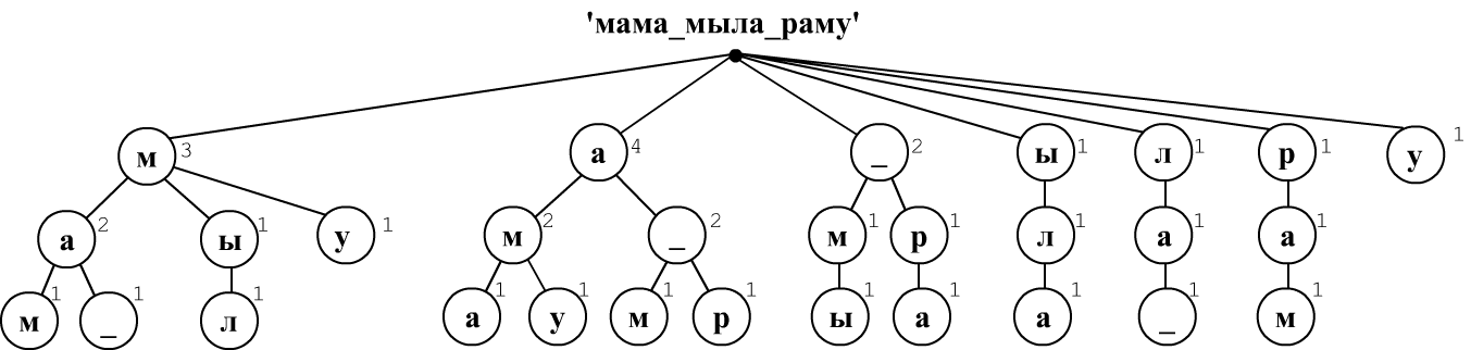
Suppose we restrict ourselves to trigrams (needed to compute joint probabilities $P(x_1,x_2,x_3)$ and conditional probabilities $P(x_1,x_2\Rightarrow x_3)$). We slide a window of three characters over the text, shifting it by one character each time. The first sequence "мам" produces the first branch of the tree root -> м -> а -> м. At each node, we record a count of one. The next sequence "ама" produces another branch emerging from the root. The third sequence "ма_" starts in the same way as the first branch, so its first two nodes increase the counters at "м" and "а", and the second node "а" then splits into two branches (for the characters "м" and "_").
It is easy to see that the conditional probability $P(\mathbf{ма}\Rightarrow \mathbf{м})$ is equal to the ratio of the count in the lower node "м" to the count in the preceding node "a", that is 1/2=0.5. The joint probability $P(\mathbf{мам})$ is equal to the ratio of the count in the last node to the total number of sequences of length 3. The same tree also provides shorter conditional or joint probabilities: $P(\mathbf{м} \Rightarrow \mathbf{а}) = P(\mathbf{ма})/P(\mathbf{а})=2/3$.
In Python, we will store each node as a vocabulary of all outgoing branches with the indication of the number count of hits into this branch from the root: words = { word: [count, words], ...}. The word vocabulary has the same structure. For example, the tree above begins as follows:
{'м': [3, {'а': [2, {'м': [1, {}],
                     '_': [1, {}]  }],
           'ы': [1, {'л': [1, {}]}  ]]
          }
      ],
  ...
}
NGramsCounter class
Let's introduce the NGramsCounter class, which counts conditional and joint probabilities up to the maximum depth order. Words can be characters, strings, or numbers (word indices).
class NGramsCounter:
    def __init__(self, order = 1):
        self.order = order           # tree depth (max n-gram length)
        self.root  = {}              # tree root (our vocabulary)
        self.ngrams= [0]*(order+1)   # number of n-grams of length n=1,2,...,order
The add method adds new samples from the word list lst. If the words are characters, lst may be a string; otherwise it must be a list.
    def add(self, lst):
        for n in range(self.order):              # how many n-grams of each size are added
            self.ngrams[n+1] += max(len(lst) - n , 0)

        for i in range( len(lst) ):              # iterate over the text
            node = self.root
            for n, w in enumerate(lst[i: i+self.order]):
                if w in node: node[w][0] += 1    # this word has already appeared
                else:         node[w] = [1, {}]  # new word
                node = node[w][1]                # move to the next tree node
The prob method takes a list of words lst and returns the conditional probability P(lst[0],...,lst[len-2] => lst[len-1]), and for len==1: P(lst[0]), if cond = True or the joint probability if cond = False If the words are characters, lst may be a string; otherwise it must be a list.
    def prob(self, lst, cond=True):
        n_cur, n_prv, _ = self.counts(lst)
        if n_cur == 0:
            return 0                              # word not found - probability 0

        return n_cur/(n_prv if cond else self.ngrams[len(lst)])
The full class code (with additional checks and other methods) can be found in my_ngrams.py.
Examples of using NGramsCounter
counter = NGramsCounter(3)                      # will count 1,2,3 -grams
counter.add('мама мыла раму')                   # count character n-grams

print("vocabulary size:", len(counter.root))    # 7
print("vocabulary words:", counter.branches())  # [('м', 4), ('а', 4), ...]
print(counter.ngrams[1:])                       # [14, 13, 12] number of n-grams n=1,2,3
print(counter.unique() )                        # [7, 10, 12] unique n-grams

N1, N2, _ = counter.counts('м')                 # N1 - occurrences of 'м', N2 - text length
print("N('м'), N       = ", N1, N2)             # 4, 14
print("P('м')          = ", counter.prob('м'))  # 0.2857 = 4/14 = N1/N2

N1, N2, _ = counter.counts('ма')                # N1 - occurrences of 'ма', N2 - occurrences of 'м'
print("N('ма'),N('м')  = ", N1, N2)             # 2, 4
print("P('м=>а')       = ", counter.prob('ма')) # 0.5 = 2/4 = N1/N2

print("P(ма=>м) = ", counter.prob('мам'))       # 0.5   = 2/4  conditional
print("P(мам)   = ", counter.prob('мам', False))# 0.083 = 1/12 joint

print(counter.branches('ма'))                   # [('м', 1), (' ', 1)] what follows ма

counter.all_branches()
# [(['м', 'а', 'м'], 1), (['м', 'а', ' '], 1),... all branches
In the NGramsCounter class, probabilities are computed as a simple ratio N1/N2. For more advanced methods, you should use subclasses of the Markov class.
Language models contain an internal counter, which is filled in the add functions. However, an external counter can also be provided, which is convenient when using multiple models:
lm = MarkovLaplas(beta=1, order=3, counter=counter)

print(lm.counter.prob("ру"))                    # 0
print(lm.prob("ру"))                            # 0.125 = (0+1)/(1+7)
print(lm.perplexity("мама умыла раму"))         # 4.886
The following language models are available:
- Markov
- MarkovLaplas
- MarkovInterpolated
- MarkovLaplasInterpolated
- MarkovBackoff
