ML: Probabilistic Inference
Introduction
Even if $n$ random variables are binary, specifying their joint probability requires $2^n-1$ numbers, which becomes computationally problematic and impractical for large $n$. Belief networks or Bayesian networks are graphical models that allow for the decomposition (simplification) of the joint probability of a large number of random variables.
This paper continues the discussion of probability theory, combinatorial and Bayesian methods. First, you should look into the Introduction to Logic and the connection between logic and probability.
Bayesian network
Let's consider the joint probability function $P(X_1,...,X_n)$ for $n$ events or random variables $X_1,...,X_n$. The Chain Rule: $$ P(X_1,...,X_n) = P(X_1)\cdot P(X_1\to X_2)\cdot P(X_1,X_2\to X_3)\cdot....\cdot P(X_1,X_2,...,X_{n-1}\to X_n), $$ can be represented as a directed acyclic graph. The nodes of the graph represent random variables, and the arrows entering a node represent conditions in the chain identity. Since the order of arguments in the right-hand side can be chosen arbitrarily, there exist $n!$ various graphs describing the joint probability. Below, the first figure shows a graph for $n=4$. The remaining 23 graphs are obtained by permutations of nodes:

If some random variables are conditionally independent, the graph simplifies (some edges disappear). The second example above is for the case where $X_2$, $X_3$ are conditionally independent given $X_1$, and for $X_4$ performed $P(X_1,X_2,X_3\to X_4)=P(X_2,X_3\to X_4)$, meaning it is conditionally independent of $X_1$. In this case, the joint probability is: $$ P(X_1,X_2,X_3,X_4) = P(X_1)\,P(X_1\to X_2)\,P(X_1\to X_3)\,P(X_2,X_3\to X_4). $$
Typically, a network is constructed based on immediate causal dependencies among random variables. After it's constructed, conditional probabilities $P(X_1,...,X_k\to X)$ are assigned to each node, where $X_1,...,X_k$ - are the incoming nodes to node $X$. Then, the joint probability can be expressed as the product of all these probabilities. Having joint probabilities, you can obtain answers to any questions about compound or conditional events.
Fred and his alarm system
 Let's consider a classic example. Suppose Fred from California
has installed an alarm system in his house,
that can go off if an (Earthquake) occurs.
Let's consider a classic example. Suppose Fred from California
has installed an alarm system in his house,
that can go off if an (Earthquake) occurs.
While he's driving, he receives an (Alarm) notification.
While listening to the (Radio), he doesn't hear any earthquake reports (although there might not have been any).
What is the probability that a (Burglar) has entered the house??
The corresponding Bayesian network is shown on the right (the burglar or earthquake can directly
influence the alarm, while only the earthquake can influence the radio message).
For this network, the joint probability is:
$$
P(B,E,A,R) = P(B)\cdot P(E)\cdot P(B,E \to A)\cdot P(E\to R) = \frac{P(B,E,A)\,P(E,R)}{P(E)}.
$$
To express this, we multiply all nodes in the network. If there are no edges entering a node (above $B$ and $E$),
the multiplier will be equal to the probability of the variable: $P(B) P(E)$. For nodes with incoming edges,
the conditional probability acts as the multiplier, where the conditions are the variables from which the edges originate.
Fred knows that events $A=a$ (there was an alarm) and $R=\bar{r}$ (there was no radio message about the earthquake) occurred. He is interested in the value of the random variable $B$ (whether a burglar entered the house): $$ P(a,\bar{r}\to B) = \frac{P(B,a,\bar{r})}{P(a,\,\bar{r})}. $$ We calculate the joint probabilities in the numerator and denominator by summing the total joint probability $P(B,E,A,R)$ over the missing variables $E:\,\{e,\bar{e}\}$ и $B:\,\{b,\bar{b}\}$: $$ P(B,a,\bar{r}) = \sum_E P(B,E,a,\bar{r}),~~~~~~~~~~~~~P(a,\bar{r}) = \sum_{B,E} P(B,E,a,\bar{r}). $$ If all conditional probabilities on the graph are known, it's easy to obtain the required conditional probability by substituting the joint probability $P(B,E,A,R)$ into these equations.
Note that the events ($B$, $E$) and ($B$, $R$) are obviously unconditionally independent in this problem. The first pair is verified by summing $P(B,E,A,R)$ over $R$ (the sum of $P(E\to R)$ equals 1) and over $A$ (the sum of $P(B,E \to A)$ equals 1). As a result, we get $P(B,E)=P(B)\cdot P(E)$. Similarly, the independence of $B$ and $R$ is proved as follows: $$ P(B,R) = \sum_{E,A} P(B,E,A,R) = P(B)\cdot \sum_{E,A} P(E)\cdot P(B,E \to A)\cdot P(E\to R) = P(B)\cdot \sum_{E} P(E)\cdot P(E\to R) $$ and further: $$ P(B,R) = P(B)\cdot \sum_{E} P(E, R) = P(B)\cdot P(R). $$
Types of Bayesian networks
Let's consider a network with three nodes. If they are all connected by arrows (the first figure below), then there are no independent nodes (both in unconditional and conditional senses). If some arrows are missing, independent nodes appear.
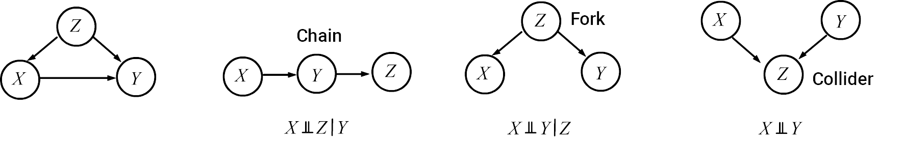
Examples with a fork and a collider were discussed in the introduction to conditional independence (ice cream and dice rolling). Let's prove conditional independence for a chain. Its corresponding joint probability is $P(X,Y,Z)~=~P(X)\,P(X\to Y)\,P(Y\to Z)=P(X,Y)\,P(Y\to Z)$. Therefore, $$ P(Y\to X,Z) = \frac{P(X,Y,Z)}{P(Y)} =\frac{P(X, Y)\,P(Y\to Z)}{P(Y)} = P(Y\to X)\,P(Y\to Z). $$
Two sets of network nodes $\mathbb{A}$ and $\mathbb{B}$ are conditionally independent given a set of node $\mathbb{C}$, if all paths between $\mathbb{A}$ and $\mathbb{B}$ are separated by nodes in $\mathbb{C}$.
A Bayesian network is called causal, if in all its connections $X_i\to X_j$, event $X_i$ s a cause for the occurrence of event $X_j$. Fred's alarm problem is an example of such a graph.
