ML: A little about entropy
Introduction
Entropy is an important measure characterizing the probability distribution and is widely used in machine learning. Before this paper, you should look into the introduction to probability theory.
Measure of uncertainty
Let's consider discrete random variables. It's useful to have a measure of uncertainty for their values. One such measure characterizing this uncertainty is the "typical" deviation from the mean value: $\sigma=\sqrt{D}$, where $D =\langle (X-X_{ср})^2 \rangle$ - dispersion. Such uncertainty of a random variable $X$ depends on both the probability distribution $\{p_1,...,p_n\}$ , and its possible values: $\{x_1,...,x_n\}$. This makes it difficult to compare the degrees of uncertainty of two variables of significantly different nature. Therefore, in some cases, it is convenient to have a measure of uncertainty that depends only on the probability distribution of the random variable.
Let's assume for simplicity that there are two events $X$ and $Y$ with probabilities $P_X$ and $P_Y$. The higher the probability of an event, the lower its uncertainty (it is more likely to occur). Therefore, we postulate that the measure of uncertainty, as a function of probability, decreases monotonically: $L(P_X) \lt L(P_Y)$ if $P_X \gt P_Y$, and for a certain event, it is equal to zero: $L(1)=0$.
Let's also postulate that the uncertainty of the joint probability $P(X,Y)=P_X\cdot P_Y$ of two independent events is equal to the sum of the uncertainties of each event: $$ L\bigr(P_X\cdot P_Y\bigr) = L\bigr(P_X\bigr)+L\bigr(P_Y\bigr) $$ These requirements fix the function up to a positive multiplier: $L(x)=-\log x$.The entropy of the probability distribution $p_i$ is, by definition, the average value of $L(p_i)$.
Entropy
Let $P=\{p_1,...,p_n\}$ be a set of $n$ non-zero probabilities. These could be probabilities of characters occurrences in text or probabilities of mutually exclusive classes in a classification model: $$ p_\alpha > 0,~~~~~~~~~~~\sum^n_{\alpha=1} p_\alpha = 1. $$ The entropy $H$ is a measure of uniformity of probabilities (the higher $H$, the closer $p_\alpha$ are to each other): $$ H(P) = - \sum^n_{\alpha=1} p_\alpha\,\log p_\alpha. $$
The natural logarithm $\ln$ or the base-2 logarithm $\log_2$ are usually chosen for the logarithm. Entropy is always positive. If all probabilities are equal: $p_\alpha=1/n$, then entropy reaches its maximum value $H_\max = \log n$. If one probability tends to 1 while the others tend to 0, then entropy tends to zero. For example, for three probabilities (with $\log=\ln$ and $\log_2$):
                       ln    log2
H(0.33, 0.33, 0.33) = 1.10 | 1.58 |
H(0.25, 0.25, 0.50) = 1.04 | 1.50 |     n:          2      3    10   100
H(0.10, 0.20, 0.70) = 0.80 | 1.16 |     ln   n:  0.69   1.10  2.30  4.61  <-  H_max ln
H(0.10, 0.10, 0.80) = 0.64 | 0.92 |     log2 n:  1.00   1.58  3.32  6.64  <-  H_max log2
H(0.01, 0.01, 0.98) = 0.11 | 0.16 |
It is worth noting that $\ln p = \log_2 p \cdot \ln 2$. Therefore, the entropy with the natural logarithm
is always equal to $0.69$ of entropy with the binary logarithm.
Entropy also characterizes the degree of "unpredictability" of mutually exclusive events with probabilities $p_\alpha$. If $n$ is small and all probabilities are small except for one, then that corresponding event almost always occurs. This situation is highly predictable (low entropy). Conversely, with a uniform distribution of probabilities, "anything can happen" (maximum entropy).
☝ The proof of the main property of entropy is conducted by finding the extremum with constraints (the method of Lagrange multipliers). The normalization condition (the sum of $p_\alpha$ equals 1) is multiplied by the parameter $\lambda$ and added to the entropy. Then we search for the extremum of $p_1,...,p_n,\lambda$: $$ H = -\sum p_\alpha\,\ln p_\alpha + \lambda\,\bigr(\sum p_\alpha- 1\bigr), ~~~~~~~\frac{\partial H}{\partial p_\alpha} = -\ln p_\alpha - 1 +\lambda = 0~~~~~=>~~~~~p_\alpha=\mathrm{const}. $$ The derivative with respect to $\lambda$ gives the normalization condition, from which it follows that $p_\alpha=1/n$.
Huffman coding
Let there be a string of characters whose probabilities are inversely proportional to powers of two. We encode each symbol with a binary number such that the code length is greater for symbols with lower probabilities. Then the entropy, using base $2$ logarithm, equals the average length in bits (per character) of the string's code.
For example, let the probabilities of symbols $\{a,b,c,d,e\}$ be $\{1/2,~1/4,~1/8,~1/16,~1/16\}$. Let's construct a binary tree with the symbols as leaves. Descending from the root (randomly choosing left or right branches), we reach these symbols with the specified probabilities (see the figure) . Then the optimal code for each symbol will be the code of the path to it in the tree ($0$ - for the left branch, $1$ - for the right branch):
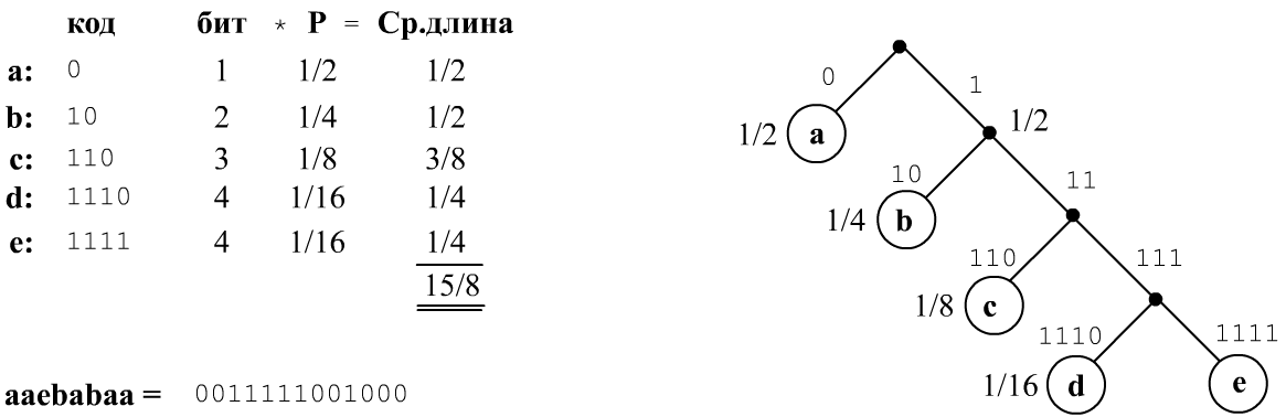
If $p_b = 1/2^b$, then $b = -\log_2 p_b$ equals the number of bits (steps from the root to the leaf). Accordingly, the average length per symbol $b\,p_b$ equals the entropy of the text.
This code is a prefix code known as Huffman coding and does not require a delimiter symbol (a binary sequence is uniquely decoded). When probabilities are not inverse powers of two, it is also possible to construct a binary tree following the algorithm below.
Initially, select two symbols with the smallest probabilities from the list and merge them into a binary branch
(in this case, d,e).
Then remove these symbols from the list and replace them with the root of their branch (as a dummy symbol)
with their combined probability.
Repeat this procedure until only one node (the root of the binary tree) remains in the list.
The average length of the Huffman code per symbol is greater than or equal to the entropy $H$ of the symbol probability distribution and less than $H_{\max}=\log_2 n$. The length of the code for each symbol usually (but not always) equals the integer part of $-\log_2 p_\alpha$.
Cross-entropy
Let's consider two sets of probabilities $P=\{p_1,...,p_n\}$ and $Q=\{q_1,...,q_n\}$. The degree of divergence between these distributions is characterized by cross-entropy: $$ H(P,Q) = -\sum^n_{\alpha=1} p_\alpha\,\ln q_\alpha. $$
It reaches a minimum when the distributions coincide $p_\alpha=q_\alpha$ (this is also proven similarly to entropy). Cross-entropy can be easily calculated in Python using the numpy library:
import numpy as np

p = np.array([0.1, 0.2, 0.7])
q = np.array([0.7, 0.1, 0.2])

H = - p @ np.log(q)
Here are examples of cross-entropy:
                                    Q              H(P,Q)
                           [0.33, 0.33, 0.33]      1.10
                           [0.25, 0.25, 0.50]      0.90
P = [0.10, 0.20, 0.70]     [0.10, 0.20, 0.70]      0.80
                           [0.10, 0.10, 0.80]      0.85
                           [0.70, 0.10, 0.20]      1.62
Note that for any $P,Q$ the inequality $H(P) \le H(P,Q)$ holds.
Cross-entropy is directly related to Kullback–Leibler divergence:
$$
D_{KL}(P,Q) = \sum^n_{\alpha=1} p_\alpha \ln \frac{p_\alpha}{q_\alpha} = H(P,Q)-H(P).
$$
This distance is always non-negative and equals zero when the probability distributions $P$ and $Q$ coincide.
Unlike typical metrics, this distance is asymmetric: $D_{KL}(P,Q)\neq D_{KL}(Q,P)$.
Conditional entropy
Let there be a vocabulary $\mathcal{V}=\{w^{(1)},...,w^{(\text{V})}\}$, consisting of $\text{V}=|\mathcal{V}|$ words (or symbols). A sequence $\mathcal{T}= w_1\,w_2....\,w_N$, where $w_i\in \mathcal{V}$ forms a text of length $N=\mathrm{len}(\mathcal{T})$. .
For each word we know $\text{V}$ probabilities $P(w_i)$ and $\text{V}^2$ conditional probabilities $P(w_i\to w_j)$. Then we can define conditional entropy as follows: $$ H_1 = - \sum_i P\bigr(w^{(i)}\bigr)~~\sum_j P\bigr(w^{(i)}\to w^{(j)}\bigr)\,\log P\bigr(w^{(i)}\to w^{(j)}\bigr). $$ Similarly, using $P(w^{(i)},w^{(j)})$ and $P(w^{(i)},w^{(j)} \to w^{(k)})$, we can define the second-order conditional entropy $H_2$, and so on.Perplexity
A probabilistic language model for a given word $w$, based on its context $\{\mathcal{T} - w\}$ (the text $\mathcal{T}$ without the word $w$) or based on the preceding words to $w$ predicts the probability of that word: $P(w|\mathcal{T} - w)$. One of the metrics for evaluating different models is perplexity. The lower the perplexity, the better the model.
The perplexity of a text $\mathcal{T}$ of length $N=\mathrm{len}(\mathcal{T})$ is defined as: $$ \mathcal{P} = \exp\Bigr( -\frac{1}{N}\,\sum^{N}_{i=1} \ln P(w_i|\mathcal{T}-w_i) \Bigr). $$
If the probabilities $P(w_i|\mathcal{T}-w_i)$ are estimated based on the preceding $w_i$ history
$P(w_i|w_1...w_{i-1})$
then, by the chain rule, we have (the sum of logarithms equals the logarithm of the product):
$\mathcal{P}=\exp(-\ln P(w_1...w_n)/N)$, or:
$$
\mathcal{P} = P(w_1,...,w_N)^{-1/N} \equiv \sqrt[N]{\frac{1}{P(w_1,...,w_N)}}.
$$
The higher the joint probability of the word sequence, the lower the perplexity.
It is important to remember that the language model should return "honest," unit-normalized
word probabilities $P(w_i|\mathcal{T}-w_i)$.
It means the sum of such probabilities for all words in the vocabulary
should be equal to one. If this is not the case, the perplexity may be unreasonably underestimated
(for example, when the model returns 1 for every word in the vocabulary).
The simplest language model, regardless of context, predicts the unconditional probability of a word: $P(w|\mathcal{T} - w) = P(w)$. In this case, the word $w^{(i)}$ will appear $N^{(i)} = P(w^{(i)})\cdot N$ times in the sum, and the perplexity is equal to the exponent of the entropy of the word probabilities: $$ \mathcal{P}_{1} = \exp\Bigr( -\sum^{n}_{\alpha=1} P\bigr(w^{(\alpha)}\bigr)\,\ln P\bigr(w^{(\alpha)}\bigr) \Bigr) ~=~ e^{H(P)}, $$ where $\mathcal{V}=\{w^{(1)},...,w^{(n)}\}$ is the vocabulary of $n$ words. When all probabilities in the model are equal to $P(w)=1/n$, the perplexity equals the size of the vocabulary (the number of different words): $\mathcal{P}_0 = n$. The minimum value of perplexity is 1. Perplexity, unlike entropy, does not depend on the base of the logarithm (you can replace $\ln\mapsto \log_2$ and $e\mapsto 2$).
Sometimes perplexity is interpreted as the degree of branching in the text (how many possible branches exist for the next word, weighted by the probabilities of these branches).
The entropy of the vocabulary depends on its size. Below are the entropy values (natural logarithm), whose probabilities are calculated on the same English text for various vocabulary sizes n (words not in the vocabulary are replaced with the UNK token):
n:            100    1000   5000   10000    36500
H:          2.913   4.811  5.841   6.080    6.247
P = exp H:     18     123    344     437      516
Therefore, indicating the perplexity of a language model generally requires specifying the size of the vocabulary the model operates on.
Typically, a language model is built on one set of documents, while perplexity is measured on another. To avoid thematic or stylistic bias, each document is divided into training and testing parts (hold-out perplexity). If cross-entropy CE is used as the model's error metric, calculated per word, then perplexity is equal to $\mathcal{P}=\exp\text{CE}$.
There is a 1B Word Benchmark data set containing approximately 829'250'940 English words with a vocabulary of 793'471 words (in an 11 GB archive). This dataset is often used to compare various language models (see here and here). For instance, 5-gram models with interpolation yield $\mathcal{P}=67$ (1.76B parameters), LSTM + CNN INPUTS (refer to this document) achieve $\mathcal{P}=30$ (1.04B parameters), and an ensemble of models reaches $\mathcal{P}=23.7$ (2016).
Differential entropy
For continuous random variables the entropy of their probability density function $p(x)$ is defined similarly: $$ H[X] = -\int\limits_X p(x)\,\ln p(x)\,dx = - \langle \ln p(x) \rangle $$ and is called the differential entropy. Let's consider a normal (Gaussian) distribution with mean $\mu$ and dispersion $D$: $$ p(x) = \frac{1}{\sqrt{2\pi D}}\, e^{-\frac{(x-\mu)^2}{2D}}. $$ The differential entropy of this distribution is: $$ H[X] ~=~ \ln\sqrt{2\pi D} + \frac{\langle(x-\mu)^2\rangle}{2D} ~=~ \frac{1}{2}\ln (2\pi\,D\,e). $$ Please note that, unlike the entropy for discrete random variables, differential entropy can be negative (especially when $D \lt 1/2\pi e$). This is because the values of probability density (unlike probabilities) can exceed unity.
It can be shown that the normal distribution has the highest differential entropy among all distributions with the same variance (this is proven using Lagrange multiplier with two constraints - normalization of the distribution and equality of its dispersion $D$). Therefore, for any random variable: $$ \langle(x-x_{ср})^2\rangle \ge \frac{e^{2H(X)}}{2\pi e}. $$
