ML: Character and Semantic Embedding
Introduction
In machine learning, a language model predicts the probabilities of words in a text. The predicted word can be the next one: $P(w_{t+1}| ...,w_{t-1},w_t)$ or a masked one: $P(w_{t}| ...w_{t-1},?,w_{t+1},...)$. The classical approach to building language models is to use n-grams with their subsequent smoothing (Markov models). The weak point of this approach is rare n-grams, which neural networks handle quite successfully using the embedding mechanism. For example, if some combination of words does not occur in the corpus, but their vectors are aligned with more frequent words, a fairly relevant probability of the n-gram can still be obtained.
Standard embeddings, however, inherit two disadvantages from n-grams:
- lack of prior knowledge about morphology;
- absence of a mechanism for handling semantic ambiguity of words.
For example, the words "walk" and "walking" are considered unrelated when constructing the vocabulary. This again creates problems for rare words, which during training must appear in similar contexts in all their word forms (in order for their embedding vectors to become close).
Morphological variability can be addressed using classical morphological analysis, through lemmatization (reducing a word to its base form using a dictionary) or stemming (extracting the word stem by cutting off endings according to simple rules). The first method requires large morphological dictionaries and is not always unambiguous ("book" = a book - noun or to book - verb). The second method can handle unknown words but sometimes makes mistakes even with common ones (for example PorterStemmer converts "healthy" to "healthi"). Another approach is to add to the word vector the embedding vectors of its character n-grams (fastText). Finally, it is possible to go directly from the word level down to the character level (2015). This approach is considered in more detail below.
Semantic ambiguity leads to a situation where a word may have completely different meanings but is associated with the same embedding vector (for example "table" - a piece of furniture or a data table). One way to mitigate this problem is through context-dependent vectorization such as ELMo, which is also discussed in this document.
Morphological analysis
Let's first consider the tools used in classical morphological analysis. The standard stemming algorithm for the English language is the Porter Stemmer. Its implementation is available in the nltk library:
import nltk

ps = nltk.stem.PorterStemmer()

for w in ["looked", "decided",  "got",  "are", "parents", "feet",  "unhealthy"]:
    print(ps.stem(w), end=", ")
         # look, decid, got, are, parent, feet, unhealthi
The same library also contains a lemmatizer based on the WordNet dictionary. For correct operation it requires the expected part of speech (the default is a noun 'n'):
nltk.download('wordnet')
wn = nltk.WordNetLemmatizer()

for p in ['n', 'v']:
    for w in ["looked", "decided",  "got",  "are", "parents", "feet",  "unhealthy"]:
        print(wn.lemmatize(w, pos=p), end=", ")
    print()
             # looked, decided, got, are, parent, foot, unhealthy
             # look,   decide,  get, be,  parent, feet, unhealthy
Other libraries that perform lemmatization are listed in this review.
Character embedding
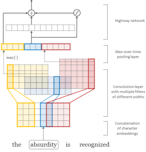 In the paper Kim Y., et al. (2015)
it was proposed to obtain word embeddings from the embeddings of their characters.
For this purpose, convolutional layers (CNN) and a max-pooling layer are used (details are shown in the figure on the right and described below).
In the paper Kim Y., et al. (2015)
it was proposed to obtain word embeddings from the embeddings of their characters.
For this purpose, convolutional layers (CNN) and a max-pooling layer are used (details are shown in the figure on the right and described below).
Let the number of characters in a language be C, and each character is assigned an embedding vector of dimension E. Then a word consisting of L characters $c_1,...,c_L$ is represented by a matrix $\mathbf{C}$ of shape (E,L) (character vectors are arranged in columns). A CNN filter $\mathbf{H}$ of shape (E,W) with width W is applied to this matrix, after which a bias $b$ is added and the result is passed through an activation function: $$ \mathbf{f}[i]= \tanh\bigr( \{\mathbf{C}[:,\,i:i+W]\odot\mathbf{H}\}.\text{sum}() + b \bigr), $$ where $\odot$ denotes element-wise matrix multiplication (without convolution). As a result, a feature vector $\mathbf{f}$ of dimension (L-W+1) is obtained. A max-pooling operation is then applied to this vector, i.e., its maximum component is selected. These values from all filters are concatenated into the final word embedding vector. Its dimensionality equals the number of filters and does not depend on their widths (each filter produces one feature). It is assumed that filters with different widths correspond to different character n-grams.
In the figure on the right, the word "absurdity" (L=9, E=4) is processed using 12 filters: 4 yellow filters (W=3), 3 blue filters (W=2) and 5 red filters (W=4). The convolution results are arranged row-wise as vectors.
To enable batch training, the authors made all words have the same length by filling missing characters with zeros (zero-padding). In addition, each word was surrounded by special start and end characters (In addition, each word was surrounded by special start and end characters). In the large model (LSTM-Char-Large) the following filter widths were used: W = [1, 2, 3, 4, 5, 6, 7] with the number of filters for each width F = [50, 100, 150, 200, 200, 200, 200] (a total of 1100 filters, which corresponds to the dimensionality of the word embedding). The smaller model (LSTM-Char-Small) contained 525 filters.
The resulting word vector $\mathbf{x}$ is then passed through a fully connected highway network (see below). The embedding vectors at its output were used by the authors to build a language model. For this purpose, the next word in a sequence was predicted using a stack of unidirectional LSTM recurrent layers. If any words could appear at the input of the model (thanks to character embeddings), then at the output of the recurrent network there was a fully connected layer with the number of neurons equal to the size of a fixed vocabulary. After that, as usual, the softmax function produced word probabilities.
Analysis based on nearest neighbors shows that the embedding vector after the convolutional network mainly reflects the character representation of the word, i.e., its morphology (which is expected). After the highway network, the vector becomes less dependent on the word form and starts to contain semantic (context-independent) features.
☝ A fully connected highway network (2015) consists of a stack of layers of the following form: $$ \mathbf{x}' = \mathbf{t}\odot g(\mathbf{x}\cdot\mathbf{W}+\mathbf{b}) + (\mathbf{1}-\mathbf{t})\odot \mathbf{x}, ~~~~~~~~~~~~~~~ \mathbf{t}=\sigma(\mathbf{x}\cdot\mathbf{W}_T+\mathbf{b}_T). $$ The matrices $\mathbf{W},\,\mathbf{W}_T$ are square, and therefore the output dimension $\mathbf{x}'$ matches the input dimension $\mathbf{x}$. In this network, the output of a standard fully connected layer with activation function $g$ (for example ReLU) is mixed with its input. The mixing weights $\mathbf{t}$ are determined by the transform gate, while $\mathbf{1}-\mathbf{t}$ correspond to the carry gate. By analogy with LSTM, this network allows certain features (components of $\mathbf{x}$) to pass from input to output unchanged.
Types of language models and RNN
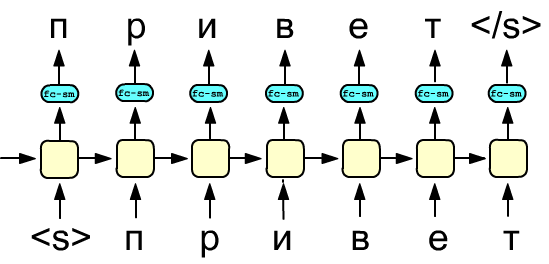 Suppose there is a sequence of $N$ tokens (words or characters): $w_1,...,w_N$.
A forward language model estimates probabilities
based on the left-to-right history (Markov chain rule):
$$
p(w_1,...,w_N) = \prod^N_{k=1} p(w_k|w_1...w_{k-1}).
$$
Suppose there is a sequence of $N$ tokens (words or characters): $w_1,...,w_N$.
A forward language model estimates probabilities
based on the left-to-right history (Markov chain rule):
$$
p(w_1,...,w_N) = \prod^N_{k=1} p(w_k|w_1...w_{k-1}).
$$
The conditional probabilities $p(w_k|w_1,...,w_{k-1})$ can be obtained using a stack of $L$ recurrent layers with indices $j=[1...L]$. Let $h_{kj}$ denote the hidden state of the $k$-th cell in the $j$-th layer. If context-independent word vectors (which do not yet contain contextual information) are fed into the first layer, then at the cell $h_{kL}$ of the final layer (after a fully connected layer and the softmax function) a probability distribution for the word $w_{k+1}$ is obtained.
The figure on the right shows the simplest version of such a network with a single recurrent layer. The yellow blocks represent LSTM or GRU cells, whose hidden state is passed both to the output and to the next cell. The blue block is a fully connected layer (fc), followed by a softmax function (sm) that produces token probabilities. The values of the input (bottom) and output (top) are shown during the teacher forcing training process. During backpropagation, the loss can be calculated either across all outputs or only across several of the last ones (after sufficient information about the sequence has been accumulated).
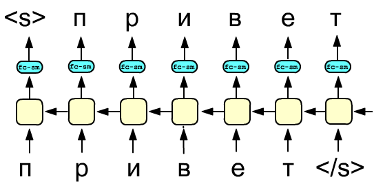 Similarly, prediction based on future context can also be used:
$$
p(w_1,...,w_N) = \prod^N_{k=1} p(w_k|w_{k+1}...w_{N}),
$$
which can also be modeled using recurrent layers, but with the hidden states flowing in the reverse direction.
Note that if in the forward network the predicted sequence (the layer output) is shifted to the left,
then for the backward flow it must be shifted to the right.
Similarly, prediction based on future context can also be used:
$$
p(w_1,...,w_N) = \prod^N_{k=1} p(w_k|w_{k+1}...w_{N}),
$$
which can also be modeled using recurrent layers, but with the hidden states flowing in the reverse direction.
Note that if in the forward network the predicted sequence (the layer output) is shifted to the left,
then for the backward flow it must be shifted to the right.
Finally, a bidirectional recurrent network, based on two opposite RNN layers, can maximize the following quantity: $$ \sum^N_{k=1}\Bigr[ \log\,p(w_k|w_1...w_{k-1}; \overrightarrow{\Theta\,}_f )+ \log\,p(w_k|w_{k+1}...w_{N}; \overleftarrow{\Theta}_b) \Bigr], $$ where the symbol $\overrightarrow{\Theta\,}_f$ denotes the parameters of the RNN cell connected from left to right, and $\overleftarrow{\Theta\,}_b$ denotes those connected from right to left. However, it is not possible to directly use a bidirectional network to construct such a language model. Some modifications are required.
Training on unlabeled data
The first figure below shows the input and output values of a bidirectional recurrent network during its forced training. The lower layer predicts the next token, while the upper layer predicts the previous one. This architecture is not suitable for text generation during inference. However, it is often necessary to obtain an integrated representation of a text, for example for sentiment analysis or for deriving a morphological vector of a word from the embedding vectors of its characters. In such cases, the bidirectional model is trained on unlabeled data to predict a shifted sequence as shown in the figure. During the inference stage, a sequence of tokens is fed into the network, and the hidden states of the layers (all of them or only the final ones) are concatenated. The resulting vector is then used to solve specific tasks. For example, in sentiment analysis this vector can be passed through a fully connected layer whose weights are trained on labeled data.
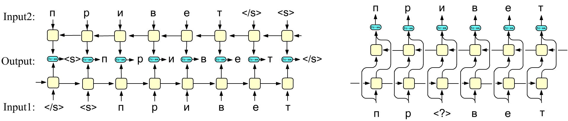
Another training strategy is shown on the right. This approach was used in the architecture of BERT (although instead of recurrent layers it uses a transformer encoder). In this method, a standard bidirectional network (possibly consisting of multiple layers) must reproduce the input sequence at the output without bias during training. At the same time, some tokens in the input sequence are "masked", i.e., replaced with a special token (in the figure this is <?>). Training on unlabeled data in this way forms a language model that can later be applied to various downstream tasks.
Finally, it is possible to train two networks independently (one processing the sequence from left to right, and the other from right to left). And then concatenate their outputs. The concatenation of the outputs from the corresponding forward and backward layers of each pair of cells (the vector before the fc-sm block) can be used as acontext-dependent token embedding. Indeed, these hidden states contain information not only about the current input token but also about the entire sequence.
Embedding mixture
To construct a morphological word embedding vector, in addition to convolutional networks, recurrent networks can also be used. For this purpose, a bidirectional network (typically a single-layer one) is employed. Character embedding vectors are fed into its input. During training, this "morphological model" learns to predict, for example, a masked character (as shown in the second figure above). After training, the concatenation of the final hidden states from each direction is taken (these states encode the word "from start to end" and "from end to start").
Since this type of embedding focuses only on morphology, it is usually combined with a standard "semantic" embedding. In the simplest case, this is done by concatenating the morphological and semantic embedding vectors. If their dimensions match, they can also be summed. The latter approach is particularly useful for rare words. Even if their semantic embedding is poorly trained (for example, when a word rarely appears in a specific form), adding it to the morphological vector makes it closer to the embedding of the base form of the word.
Naturally, after pretraining the morphological and semantic embeddings independently, they can be jointly fine-tuned.
Typically, the model outputs an index of a word from a fixed vocabulary. However, it is also possible for the model to generate the character sequence of the word instead. In this case, the word vector (after passing through the model) is fed into, for example, a unidirectional recurrent network, which is trained to produce the corresponding sequence of characters.
ELMo
ELMo (Embeddings from Language Models) is an embedding method that incorporates sentence context, thereby resolving the semantic ambiguity inherent in standard embeddings. In this approach, a language model is built by training a stack of bidirectional recurrent layers. The trained network is then used as a "provider" of context-dependent word embedding vectors. These vectors are computed as a weighted sum of the hidden states from all layers, where the weights are trainable parameters specific to the downstream task. Let's examine this idea in more detail.
Assume we have a stack of $L$ bidirectional recurrent layers. Denote the standard (context-independent) embedding vector of the $k$-th word, which is fed into the $k$-th cell of the first layer, as $\mathbf{h}_{k0}$. Let the concatenation of the hidden states of the $k$-th cell in the $j$-th bidirectional layer be: $\mathbf{h}_{kj}=[\mathbf{h}^\rightarrow_{kj},\, \mathbf{h}^\leftarrow_{kj}]$, where $\mathbf{h}^\rightarrow_{kj}$ corresponds to the forward pass, and $\mathbf{h}^\leftarrow_{kj}$ corresponds to the backward pass. The context-dependent embedding vector is defined as a linear combination of the hidden states from all layers:
$$ \mathbf{v}_k = \gamma \sum^L_{j=0} s_j\,\mathbf{h}_{kj},~~~~~~~~~~~~~~~~~~~\sum^N_{j=0} s_j = 1. $$ The coefficients $s_j$ sum to one (enforced via the softmax function), and $\gamma$ is a global scaling factor.The network is first trained on an unlabeled text corpus to predict words. After training, the layer weights are frozen, and the network is used to produce the components $\mathbf{h}_{kj}$ for the formula above. The parameters $s_j$ and $\gamma$ are then optimized using labeled data for a specific downstream task.
References
Articles
- 2015:
Srivastava, R. K., et.al
"Training Very Deep Networks"
- highway network architecture. - 2015: Kim Y., et al.
"Character-Aware Neural Language Models"
- character-level word embedding. - 2016: Jozefowicz R., et al.
"Exploring the Limits of Language Modeling"
- study of language models by Google Brain, including character-based embeddings at both input and output. - 2018 :
Peters M.E., et.al
"Deep contextualized word representations"
- the ELMo model.
