ML: Embedding Layer in Keras
Introduction
In neural networks, there is a special type of layer called Embedding, which takes word indices as input and outputs their vector representations (random at the start of training):
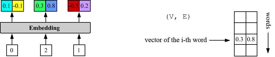
Above, VEC_DIM = 2 and the layer has three inputs (inputs = 3). The first word has index 0, the second 2, and the third 1. The Embedding layer stores a matrix of shape (DIC_SIZE, VEC_DIM), from which, given an input number i, it outputs the i-th row.
Accompanying file: NN_Embedding_Layer.ipynb. General theory of word vectorization can be found in this document. The Embedding layer in the PyTorch library is described here.
Embedding in Keras
As in many other layers of the Keras library, when creating an Embedding layer, it is not necessary to specify the batch size (batch_size - the number of examples over which the loss is computed). It is mandatory to specify the vocabulary size VOC_SIZE and the vector dimension VEC_DIM (these determine the size of the embedding matrix). Optionally, you can also specify the number of inputs:
VOC_SIZE = 5       # number of words in the vocabulary
VEC_DIM  = 2       # vector space dimension
inputs   = 3       # number of inputs (number of integers)

m = Sequential()
m.add(Embedding(input_dim = VOC_SIZE, output_dim = VEC_DIM, input_length = inputs)
The shapes of the input and output tensors of the Embedding layer look like this:
(batch_size, inputs) => (batch_size, inputs, VEC_DIM)The layer always comes first because its input tensor contains integers: [0...VOC_SIZE-1]. The number of inputs, like the batch size, can be omitted (as they are automatically inferred from the input tensor):
m = Sequential()
m.add(Embedding(VOC_SIZE, VEC_DIM))    # variable batch size and number of inputs
For example, below batch_size=1 and inputs=1, 2:
print(m.predict([[0]]))    # (1,1)=>(1,1,2): [ [[0.01  0.025]] ]
print(m.predict([[0,4]]))  # (1,2)=>(1,2,2): [ [[0.01  0.025], [0.035 0.012]] ]
Similarly with batch_size=2 (the list of lists must be explicitly converted into a numpy tensor!):
print(m.predict(np.array([ [1,2], [3,4] ]) ))

    input1             input2
[ [[-0.044  0.029],  [ 0.01   0.038]]       sample1
  [[-0.018 -0.045],  [ 0.035  0.012]] ]     sample2
Vector matrix
In the method m.layers[0].get_weights(), as usual, there is a list of matrices with the parameters of the zero-th layer. In this case, it consists of a single matrix of shape (VOC_SIZE,VEC_DIM):
[[ 0.01   0.025]          <= the first word     id = 0
 [-0.044  0.029]
 [ 0.01   0.038]
 [-0.018 -0.045]
 [ 0.035  0.012]]         <= the last word      id = VOC_SIZE-1
Before training, the vector components are random numbers, generated by the initializer specified with embeddings_initializer (default is 'uniform': $[-0.05, 0.05]$, see initializers).
You can load a pre-trained matrix of vector components (for example, trained on another task). If it should not be updated during further training, set trainable=False:
m = Sequential()
m.add( Embedding(VOC_SIZE,VEC_DIM, weights=[embedding_matrix], trainable=False) )
Regularization and constraints
The vector components of the Embedding layer are trainable parameters. For them (as for any parameters), you can set value constraints and add regularization terms to the loss.
The embeddings_constraint parameter (default None) specifies constraints. For example:
m.add(Embedding(100,2, embeddings_constraint = keras.constraints.UnitNorm(axis=1)))will ensure that the vectors have unit norm.
The embeddings_regularizer parameter (default None) applies a softer constraint on the vector components. For this, a term is added to the loss function, e.g., the sum of squares of the components multiplied by a small constant (below 0.01). The gradient method will simultaneously try to reduce the model's prediction error and the magnitude of the components, preventing them from growing uncontrollably:
m.add(Embedding(100,2, embeddings_regularizer = keras.regularizers.l2(0.01) ))
Interaction with Dense and RNN
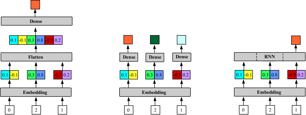
The fully connected Dense layer connects synapses to the last dimension of the previous tensor: $\sum_\alpha X_{i...j\alpha}\,W_{\alpha k}=Y_{i...jk}$. The output of the Embedding layer is a tensor of rank three, not two, with shape (batch_size, inputs, VEC_DIM). Therefore (if the vectors need to be concatenated), when connecting a Dense layer after an Embedding layer, a Flatten() layer must be inserted between them:
m = Sequential() # 5         2                        Output shape:    Params:
m.add(Embedding(VOC_SIZE, VEC_DIM, input_length=3)) # (None,3,2)       5*2 = 10
m.add(Flatten())                                    # (None,6=2+2+2)   0
m.add(Dense(1))                                     # (None,1)         3*2+1 = 7
Below, the first figure shows the architecture of this model. The number of parameters in the Embedding layer is VOC_SIZE*VEC_DIM, and for a Dense layer with one neuron (units=1), the weight matrix (inputs*VEC_DIM, 1) and the bias (a single number) gives inputs*VEC_DIM + 1 parameters.
The Flatten layer has no parameters. Its task is to make the incoming data tensor linear. It does not affect the zeroth batch axis, i.e., when Flatten() is applied to a tensor (batch_size, size1,...,sizeN), the resulting tensor is (batch_size, size1*...*sizeN):
t = keras.backend.ones((10, 2, 3, 4, 5))            # (10, 2, 3, 4, 5)
print( Flatten()(t).shape )                         # (10, 120)
If the dimensionality reduction by Flatten is not done, the model:
m = Sequential() # 5         2                        Output shape:    Params:
m.add(Embedding(VOC_SIZE, VEC_DIM, input_length=3)) # (None,3,2)       5*2 = 10
m.add(Dense(1))                                     # (None,3,1)       2+1 = 3
will combine the outputs of the Embedding layer and the weights of the Dense layer with units neurons as follows:
np.dot( (batch_size, inputs, VEC_DIM), (VEC_DIM, units) ) = (batch_size, inputs, units).
The number of parameters in the Dense layer will now be VEC_DIM+1. This means that the same weights are applied to each vector. This architecture is shown in the center figure below:
Unlike the Dense layer, recurrent layers expect vectors at their input, so the Embedding layer is connected to them directly (the third figure above):
m = Sequential() # 5         2                        Output shape:    Params:
m.add(Embedding(VOC_SIZE, 2, input_length = 3))     # (None, 3, 2)     5*2 = 10
m.add(LSTM(1))                                      # (None, 1)        4*((2+1)+1)=16
By default, the recurrent network (LSTM) has return_sequences=False, so above it returns only the hidden state (one-dimensional) of the last (third) cell.
Input masking
It is recommended to reserve the first word in the vocabulary (zero index) and not assign a meaningful word to it. Then the zero index can be used as a signal for missing input. This is useful for variable-length inputs, for example in RNNs. To use masking in the Embedding layer, set mask_zero=True. The layer will still output vectors according to the number of inputs. However, the subsequent RNN layer will ignore vectors with zero index, moving to the next cell:
m = Sequential()
m.add( Embedding(VOC_SIZE,VEC_DIM, mask_zero=True) )
m.add( SimpleRNN(1,  return_sequences=True) )

print(m.predict(np.array([ [1,0,3,0,2,0,0] ]) ))

[[[0.02 ]        # computed for 1
  [0.02 ]        # skipped (0), repeated hidden state for 1
  [0.069]        # computed for 3
  [0.069]        # skipped (0), repeated hidden state for 3
  [0.065]        # computed for 2
  [0.065]        # skipped (0), repeated hidden state for 2
  [0.065]]]      # skipped (0), repeated hidden state for 2
Usually, masked zero inputs are placed at the end of the sequence, "padding" short sentences to the maximum length with zeros.
Masking is also taken into account when computing the loss, ignoring errors from masked inputs.
