ML: Character Prediction
Introduction
Let's consider an example of predicting the next character in a text using a recurrent neural network. The source code can be found in the notebook NN_RNN_Torch_Chars.ipynb
Data preparation
As a small playground, we will use "The Tale of Tsar Saltan". We will use a fixed alphabet CHARS and include the newline character '\n' (for poetry):
CHARS  = " .абвгдежзийклмнопрстуфхцчшщъыьэюя\n"        # alphabet
charID = { c:i for i,c in enumerate(CHARS) }           # character to index
Load the text from a file, convert it to lowercase, remove double spaces, etc.:
import re

with open("saltan.txt", "r", encoding='utf-8-sig') as file:
    text = file.read()

    text = text.lower().replace('ё','e')
    text = ''.join( [c if c in CHARS else ' ' for c in text] )
    text = re.sub(' +',    ' ',  text).replace(' .', '.')
    text = re.sub('\n\s+', '\n', text)
To form the training data, we slide a window of LENGTH with a STEP over the text. The indices of characters that fall into the window are placed in X_dat. The target array Y_dat contains characters shifted one position forward:
LENGTH, STEP = 25, 25                         # story length, text step
textID = [ charID[c] for c in text ]          # text as list of indices (positions in CHARS)

num_seq  = int((len(textID)-LENGTH)/STEP)-1   # number of sequences

X_dat = torch.empty (num_seq, LENGTH, dtype=torch.long)
Y_dat = torch.empty (num_seq, LENGTH, dtype=torch.long)

for i in range(num_seq):
    X_dat[i] = torch.tensor(textID[i*STEP:   i*STEP+LENGTH],   dtype=torch.long)
    Y_dat[i] = torch.tensor(textID[i*STEP+1: i*STEP+LENGTH+1], dtype=torch.long)
The STEP is chosen equal to the window width LENGTH so that after shuffling,
validation data does not overlap with training data (see the next section).
Shuffle the data and split it into training (X_trn, Y_trn)
and validation (X_val, Y_val) sets:
idx = torch.randperm( len(X_dat) )            # shuffled list of indices
X_dat, Y_dat = X_dat[idx], Y_dat[idx]

num_trn = int(0.75*len(X_dat))                # proportion of training data
X_trn, Y_trn = X_dat[:num_trn], Y_dat[:num_trn]
X_val, Y_val = X_dat[num_trn:], Y_dat[num_trn:]
Training strategy
In principle, the network can be trained to predict Y_trn from the input X_trn, using all outputs of the recurrent layer. However, we will do it differently. We introduce a hyperparameter NUM, which is smaller than the sequence LENGTH. The network will accumulate the hidden state (history) over the first LENGTH - NUM cells. Prediction errors will be calculated only on the last NUM cells. Using NUM > 1 is useful for reducing gradient vanishing during backpropagation.
Below is a diagram of a two-layer RNN network. The first layer cells receive the text "вечерко" In reality, not just one but B examples of length L (a batch) participate in training simultaneously. Therefore, the network input is a tensor of shape (B,L) containing character indices. It passes through the Embedding layer and each character is transformed into an E-dimensional vector, resulting in a tensor of shape (B,L,E):
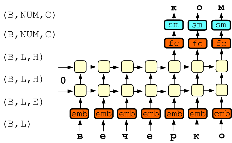
The output of the last RNN layer has shape (B,L,H), where H is the hidden state dimension. For loss calculation, only the last NUM cells are taken. Therefore, the tensor (B,NUM,H) is transformed using a fully connected layer fc (with matrix of shape (H,C)) into a tensor (B,NUM,C), where C is the number of letters in the alphabet (number of classes). After passing this tensor through the softmax function sm, for each example B and output NUM we get C numbers, which are interpreted as probabilities of a particular character (the sum of numbers after sm equals one). The prediction loss is computed as the average CrossEntropyLoss over all NUM outputs and B examples.
The model
In the model constructor we create an Embedding layer, a stack of NUM_LAYERS GRU recurrent layers, an output fully connected Linear layer, and a Dropout layer that with probability DROP zeros out components of the tensor before fc:
class Model(nn.Module):
    def __init__(self, C, E, H, LAYERS = 1, DROP = 0):
        super(Model, self).__init__()

        self.emb  = nn.Embedding(C, E, scale_grad_by_freq=True)
        self.rnn  = nn.GRU    (E, H, num_layers=LAYERS, batch_first=True, dropout=0.2)
        self.drop = nn.Dropout(DROP)
        self.fc   = nn.Linear (H*LAYERS, C)
Note the scale_grad_by_freq parameter when creating the Embedding layer. Letters in the text have substantially different probabilities. Therefore, during training more frequent characters will update their vector components more intensively than rarer ones. When scale_grad_by_freq = True, character probabilities are calculated for the current batch and the optimizer shifts vectors of rarer characters more strongly.
The forward propagation method defines the sequence of computations. The shapes of the resulting tensors are shown in comments on the right.
.   def forward(self, x, h0=None, NUM=1):       # (B,L), (1,B,H)
        x      = self.emb ( x )                 # (B,L,E)
        yr, hr = self.rnn ( x, h0 )             # (B,L,H),  (1,B,H)

        y = yr[:, -NUM:,  :]                    # (B,NUM,H) last outputs
        y = self.drop(y)
        y = self.fc(y)                          # (B,NUM,C)
        return y.transpose(1,2), hr             # (B,C,NUM), (LAYERS,B,H)
In our training strategy, the fully connected layer matrix fc is multiplied
not with the entire output tensor (B,L,H), but only with its slice
(B,NUM,H).
In addition to acceleration, this can lead to significant memory savings with a large vocabulary
(when working with words instead of characters). For example, suppose a batch has B=100 examples,
the hidden state dimension H=500
and the vocabulary size C=100'000 words.
Then the tensor of all outputs of the RNN layer
has 100*500*L elements, while the tensor after the fully connected layer
is 200 times larger: 100*100000*L. With long sequences L,
such a tensor may not even fit into GPU memory. Therefore, multiplying
all outputs of the RNN layer with the fully connected output layer fc is not advisable.
Creating a model instance is standard. If a GPU is available, the model parameters are immediately moved to its memory. The losses list will be needed later for visualizing the training error history.
E_DIM, H_DIM, NUM_LAYERS, DROP = 10, 250, 1, 0

model = Model(len(CHARS), E_DIM, H_DIM)         # model instance

gpu = torch.device("cuda:0" if torch.cuda.is_available() else "cpu")
cpu = torch.device("cpu")

model.to(gpu)
losses = []                                     # loss history for plotting
Class weights and loss function
Another way to deal with class (character) probability imbalance is to use weights that reflect the importance of the error for a given character. If all weights are the same, the network tends to predict frequent characters better than rarer ones. To reduce this effect, we calculate the frequency of each character weight, and then take its negative logarithm.
weight = torch.zeros(len(CHARS), dtype=torch.float)
for c in textID:
    weight[c] += 1

weight /= len(text)
weight = -weight.log_()
Here are the weights for the 5 most frequent and 5 rarest characters:
     ' ': 1.86   'о': 2.51   'е': 2.76   'а': 2.72   'и': 2.98
     'ю': 5.49   'щ': 6.44   'э': 7.49   'ъ': 7.49   'ф': 8.95
Using the logarithm makes the increase in weight for rare characters softer
compared to, for example, inverse probability.
Normalizing the weights is not necessary, as the loss function does it automatically.
CE_loss = nn.CrossEntropyLoss(weight.to(gpu))
Training
The training function for one epoch looks like this:
def fit(model, X,Y, batch_size=64, NUM=1, train=True):
    model.train(train)                                   # important for Dropout
    sumL, iters = 0, int(len(X)/batch_size)

    tm1 = tm()
    for it in range(iters):                                # examples split into batches

        xb = X[it*batch_size: (it+1)*batch_size].to(gpu)   # (B,L)
        yb = Y[it*batch_size: (it+1)*batch_size].to(gpu)   # (B,L)

        y, _ = model(xb, NUM=NUM)
        L    = CE_loss(y, yb[:, -NUM:])

        sumL += L.detach().item()

        if train:                                        # training mode
            optimizer.zero_grad()                        # zero gradients
            L.backward()                                 # compute gradients
            optimizer.step()                             # update parameters

        if tm() - tm1 > 1 or it+1==iters:
            print('\r', f"{100*(it+1)/iters:.0f}%  loss: {sumL/(it+1):.4f}", end='')
            tm1 = tm()

    return sumL/iters
Launching training:
from IPython.display import clear_output
import matplotlib.pyplot as plt

for epoch in range(100):
    optimizer = torch.optim.Adam(model.parameters(), lr=0.001, betas=(0.9, 0.999))

    idx = torch.randperm( len(X_trn) )     # shuffled list of indices
    X_trn = X_trn[idx]
    Y_trn = Y_trn[idx]

    L_trn, A_trn = fit(model, X_trn, Y_trn, 256, NUM = 25, train=True )
    L_val, A_val = fit(model, X_val, Y_val, 256, NUM = 25, train=False)
    losses.append([L_trn, L_val])

    clear_output(wait=True)
    plt.figure(figsize=(16,4)); plt.plot(losses); plt.legend(['trn', 'val']);  plt.show()

    print('\r', f'epoch: {epoch:d}/{len(losses)-1}  {tm()-beg:.2f}s ',
                f'loss: trn={L_trn:.4f} val={L_val:.4f}  ' )
One-hot vs Embedding
Since there are few characters in the vocabulary, we could remove the Embedding layer and use one-hot encoding instead. To do this, it is enough to set E_DIM=len(CHARS) and replace the line x = self.emb ( x ) in the forward function with:
B, L, C = len(x), x.size(1), self.fc.size(-1)
x = torch.zeros(B,L,C).scatter_(2, x.unsqueeze(2), 1.)    # (B,L,C)
x = x.transpose(0,1).contiguous()                         # (L,B,C)
Since x has shape (B,L), we first create a tensor (B,L,C) filled with zeros. The method x.unsqueeze(2) changes the tensor shape: (B,L) -> (B,L,1). The scatter_ method places ones in the last index of the tensor at the position corresponding to the value in x. Pseudocode for this method is: self[i,j, x[i,j,k]] = 1. For example:
L, C = 3, 4
x = torch.tensor([ [1,0,1],  [0,2,3] ], dtype=torch.long)
x = torch.zeros(len(x), 3, 4).scatter_(2, x.unsqueeze(2),  1.)   # (B,L,C)

[[[0., 1., 0., 0.],  [1., 0., 0., 0.],  [0., 1., 0., 0.]],
 [[1., 0., 0., 0.],  [0., 0., 1., 0.],  [0., 0., 0., 1.]]])
