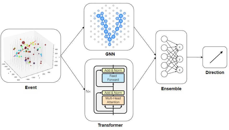
Ensemble set-up
The results of the architectures we trained (Transformer and GNN) were not strongly correlated with each other. This made it possible to form ensembles of models, which gave a significant improvement in the final metric. In addition, thanks to the remarkably large dataset provided by the organizers, additional progress in the metric could be obtained using the trained ensemble. The general architecture of the ensemble looked like:
Ensemble Models
In each architecture, several models were selected, obtained with different hyperparameters or architecture options. 80 batches were passed through these models, the results of which formed a dataset for the ensemble.
Below are the initial data of the selected models. The first column of numbers is the base metric of the competition (mean angular error). The second two columns are the azimuth error and the module of the zenith error of the model (all validations were carried out on the first 5 batches):
id   ang_err  az_err  ze_err   model
 0   0.9935   1.035   0.606  | gnn_1
 1   0.9922   1.033   0.595  | gnn_2
 2   0.9963   1.039   0.598  | gnn_3
 3   0.9954   1.018   0.612  | att_1
 4   0.9993   1.022   0.636  | att_2
---------------------------------------------------------------
     0.9846   1.021   0.540  | simple mean
The criterion for selecting models for the ensemble was the angular error and coefficients of correlations of the angular error between different models:
     0        1        2        3        4
 0            0.959    0.950    0.807    0.781
 1   0.959             0.934    0.820    0.795
 2   0.950    0.940             0.808    0.783
 3   0.807    0.820    0.808             0.940
 4   0.782    0.795    0.783    0.940
Simply averaging the vectors predicted by each model resulted in a 0.9846 error.
Next, we built an ensemble with trainable weights (the multiplier of each model): $$ \mathbf{n} = w_1\,\mathbf{n}_1 + ...+ w_5\,\mathbf{n}_5 $$ This reduced the error to 0.9827. In this case, the regression weights of the models had the form:
gnn_1: 0.934, gnn_2: 1.346, gnn_3: 0.753, att_1: 1.466, att_2: 0.477
Training Ensemble
Further advancement of the metric was achieved by a trained ensemble based on a neural network. Several architectures were considered, including a transformer and adding aggregated event features to the model outputs. However, they turned out to be no better than conventional MLP with one hidden layer. The tensor (B,N,3) was fed at the input of this network, where B is the number of examples in the batch, N is the number of models, each of which produced three components of the direction vector. This tensor was converted into dimension (B,3*N). After MLP, its dimension became equal to (B,3).
The number of neurons in the hidden layer ranged from 128 to 2048. However, all these models gave approximately the same results. For training, the best loss appeared to be the cosine between the predicted and the target vector. The learning rate was quite high lr = 1e-3 - 1e-4 and the Adam optimizer was used.
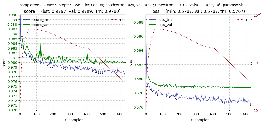
The best metric, as determined by the validation on the first 5 batches, gave the result 0.9796. Below are some typical learning curves: