Transformer
 The model, which we named "Transformer", is a combination of architectures that include fully connected blocks, an attention mechanism, and a recurrent layer.
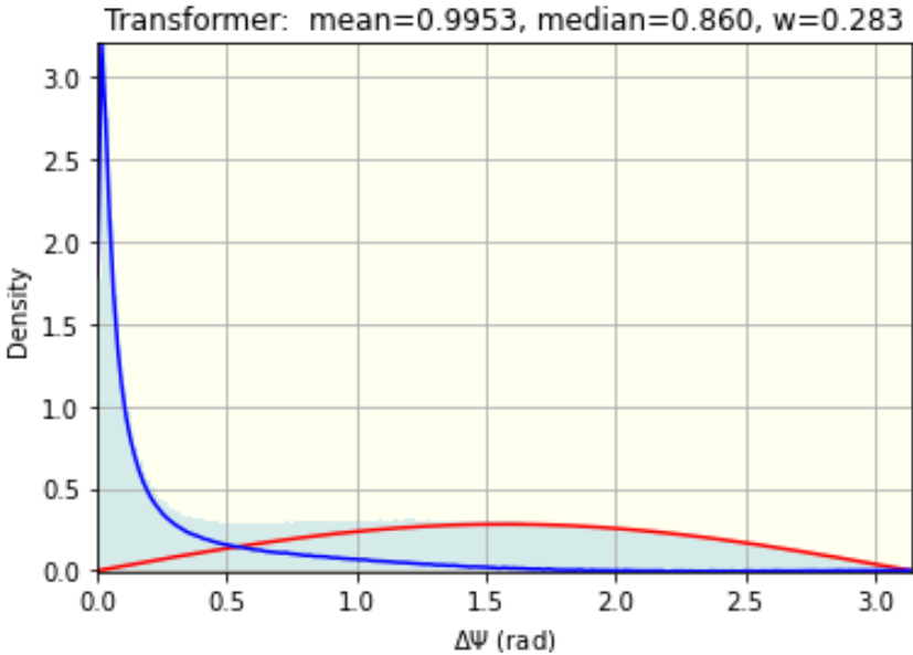
The typical metric achieved by this model was 0.995.
At the same time, the more parameters the model has, the more the metric can be improved.
However, moving forward with a bigger transformer would require a pair of spare A100 GPUs, which we didn't have :)
The model, which we named "Transformer", is a combination of architectures that include fully connected blocks, an attention mechanism, and a recurrent layer.
The typical metric achieved by this model was 0.995.
At the same time, the more parameters the model has, the more the metric can be improved.
However, moving forward with a bigger transformer would require a pair of spare A100 GPUs, which we didn't have :)
The general architecture of the Transformer model looked like this. It receives two tensors as input: (B,T,PF) and (B,EF), where B is the index of the sample in the minibatch and T is the index of the pulse number in the sequence. Each pulse was characterized by PF=9 features. The second tensor (B,EF) characterized the properties of the entire event with EF more features. These features were calculated for all pulses of the event (24 features) and inaddition only for the pulses marked with the auxiliary=0 flag (we'll shorten it to "aux"), 24 more.
In some modifications of the architecture, aggregated features with aux=0, using a fully connected MLP block (multilayer perceptron) with one hidden layer, were compressed to a smaller dimension and then combined with the pulse feature tensor (B,T,PF). The motivation for compression is related to the fact that the number of event features (24) was significantly greater than the number of more significant pulse features (9). In other architectures, only features of pulses were used.
After concatenation, the resulting tensor (B,T,F) was fed to the second MLP block (below the Feature Generator). Its task was to increase the number of features to E=128. The resulting tensor (B,T,E) was fed to a chain of 10–12 transformer blocks. Each pulse, as a result of the mechanism of attention, "interacted" with all the pulses in the sequence. As a result of the work of the transformer, the pulses received new features in the space of the same dimension.
Next, the Integrator block converted the transformer output tensor (B,T,E) into a tensor of (B,E') dimensions. At the initial stage of training, the concatenation of the operation of averaging and obtaining the maximum according to the features of all pulses acted as the Integrator block. At the final stage, this block was replaced by an RNN layer integrating the event pulses. One unidirectional recurrent layer with GRU cells was chosen as RNN. In this case, the pulses of the event were sorted in reverse order by time. As a result, the input of the last GRU cell (the output of which was used by the Integrator) received the most significant, that is the first, pulse.
The event feature tensor for all pulses and pulses with aux=0 was attached to the (B,E') tensor obtained after the Integrator. The resulting tensor (B,E'+2*EF) was fed to an MLP whose three outputs were Cartesian components of the direction vector predicted by the regression model.
The transformer had a standard architecture with 16 heads in the attention block and trainable weights on skip-connections:
Pulse and event features
As an "embedding" element of the sequence we selected 9 features of the pulse. The first 6 determine the spatial position of the pulse:- \(x,y,z\) - sensor coordinates;
- \(\text{core}\) - pulses belonging to the core strings (\(0,1\));
- \(a\) - coefficient of absorption of light by ice at sensor's depth;
- \(\rho = \sqrt{x^2+y^2}\) - distance from the central axis (taking into account edge effects).
- \(t\) - time;
- \(q\) - charge;
- \(\text{aux}\) - auxiliary feature (\(0,1\)); when aggregating pulses by DOM - \(\text{aux}\in [0...1]\);
def get_sensors():
    df = pd.read_csv(PATH / "sensor_geometry.csv")
    df['line_id'] = df.sensor_id // 60 + 1                 # string id
    df['core']    = (df.line_id > 78).astype(np.float32)   # sensor from DeepCore
    df.x = ( df.x * 1e-3 ).astype(np.float32)              # distances in kilometers
    df.y = ( df.y * 1e-3 ).astype(np.float32)
    df.z = ( df.z * 1e-3 ).astype(np.float32)

    from scipy.interpolate import interp1d                 # add absorption
    phys = pd.read_csv(PATH_PHYS / "scattering_and_absorption.csv")
    phys.z = (phys.z * 1e-3).astype(np.float32)
    phys.a = (phys.a * 1e-2).astype(np.float32)
    interp = interp1d(phys.z, phys.a)
    df['a'] = interp(df.z)

    df['r'] = np.sqrt(df.x**2 + df.y**2)

    return df[['sensor_id', 'line_id', 'core', 'x', 'y', 'z', 'a', 'r']]
The six DOM features acted as components of the Embedding layer.
It was frozen at the beginning of the training: requires_grad_(False).
At the end of the training, this layer was made trainable to "correct" the DOM coordinates.
The dynamic pulse features \(t,q,\text{aux}\) were concatenated with DOM features. Time was normalized so that the speed of light was equal to unity. In addition, the beginning of the time axis was shifted to zero for the first pulse:
def prepare_batch(df, verbose=True, drop_aux = DROP_AUX, doms_agg = DOMS_AGG):
    #...
    times = df.groupby('event_id').agg( t_min = ('t', 'min') )
    df = df.merge(times, left_on='event_id', right_index=True, how='left')
    df.t = (( df.t - df.t_min ) * 0.299792458e-3 ).astype(np.float32)
Event duration
The amount of memory required to train the transformer grows quadratically with the number of elements of the sequence T. A computational graph of size 3*B*H*T*T is stored in each of the L blocks (for gradient backpropagation). Therefore, for example, with T=1024, H=16 (number of heads), B=256 (batch size) and L=10 blocks, just the computational graph of the transformer requires about 12Gb. Therefore, at the initial stages of training, pulses were aggregated on the sensor to reduce T. The time of the first pulse (on this sensor) was taken as the time, and the total charge was taken as the charge.
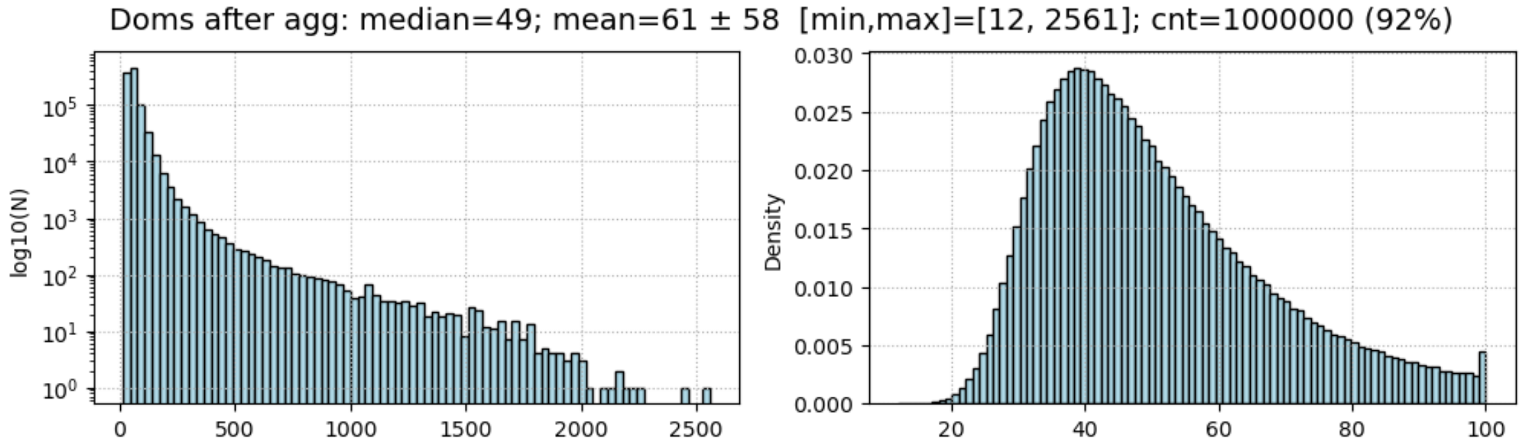
In addition to DOM aggregation, the latest pulses in long events were discarded. To do this, sorting was done - first by aux, then by time. The number of retained pulses at different stages of training was different. In the beginning it was relatively small T=64. At the end of training, it increased to T=256, which usually gave a few extra points to the metric. The choice of the number of active sensors was determined by the following histogram (the median value of the number of DOMs is 49):
However, at the end of the competition, we abandoned the aggregation of pulses by DOM. This reduced the error by 3-4 points, although it required significant additional training of the model on A100 cards on Colab-Pro.
Event features
Various integral characteristics were chosen as features of an event, the meaning of which should be clear from the following code:
df = df.groupby('event_id').agg(          # for all pulses, for any aux
    tot      = ('t',        'count'),
    t_med    = ('t',        'median'),
    t        = ('t',        'mean'),
    x        = ('x',        'mean'),
    y        = ('y',        'mean'),
    z        = ('z',        'mean'),
    stdT     = ('t',        'std'),
    stdX     = ('x',        'std'),
    stdY     = ('y',        'std'),
    stdZ     = ('z',        'std'),
    xt       = ('xt',       'mean'),
    yt       = ('yt',       'mean'),
    zt       = ('zt',       'mean'),
    tt       = ('tt',       'mean'),
    q        = ('q',        'mean' ),
    q_min    = ('q',        'min' ),
    q_max    = ('q',        'max' ),
    q_med    = ('q',        'median' ),
    aux      = ('aux',      'mean' ),
    core     = ('core',     'mean' ),
    lines    = ('line_id',  'nunique' ),
    doms     = ('sensor_id','nunique' ),
)
We also experimented with other features of the event, including "center of mass" in charge and
"inertia tensor" by charge.
Implementation details
To implement the transformer we used our own implementation, which is a derivative of a small library by Andrej Karpathy. This code, along with the rest of the notebooks, is posted on github QuData. The main difference from the base implementation is the use of skip-connection multipliers, which can be trained.
Below is the structure of the parameters of one of the models included in the ensemble:
===================================================================================
Layer (type:depth-idx)                        Param #                   Trainable
===================================================================================
Regression                                    --                        Partial
├─Model: 1-1                                  --                        Partial
│    └─FeatureGenerator: 2-1                  --                        Partial
│    │    └─Embedding: 3-1                    (30,960)                  False
│    │    └─MLP: 3-2                          --                        True
│    │    │    └─Linear: 4-1                  2,560                     True
│    │    │    └─Linear: 4-2                  32,896                    True
│    └─Transformer: 2-2                       --                        True
│    │    └─ModuleList: 3-3                   --                        True
│    │    │    └─TransformerBlock: 4-3        2                         True
│    │    │    │    └─LayerNorm: 5-1          256                       True
│    │    │    │    └─SelfAttention: 5-2      66,048                    True
│    │    │    │    └─LayerNorm: 5-3          256                       True
│    │    │    │    └─MLP: 5-4                131,712                   True
│    │    │    └─TransformerBlock: 4-4        2                         True
               ...                            [ total 12 blocks ]
│    │    └─Dropout: 3-4                      --                        --
│    │    └─LayerNorm: 3-5                    256                       True
│    └─Summator: 2-3                          --                        True
│    │    └─LayerNorm: 3-6                    256                       True
│    │    └─GRU: 3-7                          296,448                   True
│    └─MLP: 2-4                               --                        True
│    │    └─Linear: 3-8                       624,640                   True
│    │    └─Linear: 3-9                       6,147                     True
===================================================================================
Total params: 3,373,451
Trainable params: 3,342,491
Non-trainable params: 30,960
Each block of the architecture was designed as a separate module:
class FeatureGenerator
class Transformer
class Integrator
All of them were collected in the Model class inside which there was an output regression MLP, and the error and other metrics were calculated. To be able to experiment with different architectures, a set of flags was used (is_abs, is_rho, is_fin, is_emb, etc.). Depending on their values, one or another architecture of the model was formed. Here is an example of the first block for generating features fed to the transformer:
class FeatureGenerator(nn.Module):
    def __init__(self, cfg, doms, V=5160):
        """
        Feature generator.
        Gets the original pulse and event features, outputs a tensor (B,T,E).
        V - number of sensors (embedding vocab) from sensors_df
        """
        super().__init__()

        dom_feat = 4                       # {x,y,z,core}
        if cfg.is_abs and not cfg.is_rho:  # {x,y,z,core,a}
            dom_feat = 5
        else:                              # {x,y,z,core,a,r}
            dom_feat = 6

        self.dom = nn.Embedding(V,dom_feat,_weight=doms[:,:dom_feat]).requires_grad_(False)
        self.emb = nn.Embedding(V,cfg.SE) if cfg.is_emb else None # sensor embedding

        self.fin = MLP(dict(input=24, hidden=64, output=7)) if cfg.is_fin else None

        F = dom_feat+cfg.F   # {x,y,z,core [,a]} + {t,q,aux}
        if cfg.is_fin:
            F += 7
        if cfg.is_emb:
            F += cfg.SE      # add sensor SE embedding
        self.mlp = MLP(dict(input=F, hidden=cfg.Hin, output=cfg.n_embd)) \
                   if cfg.Hin > 0 else nn.Linear(F, cfg.n_embd)

    def forward(self, SENSOR_ID, FEAT, AGG):
        s  = self.dom(SENSOR_ID)                  # (B,T,5)   x,y,z,core,a,r
        if self.emb is None:
            x  = torch.cat([s, FEAT], dim=2)      # (B,T,E0)  pulse feat+'aux','q','t'
            if self.fin is not None:
                T = x.shape[1]
                f = self.fin(AGG[:, 24:])         # (B,7)
                f = f.unsqueeze(1).expand(-1,T,-1)# (B,T,7)
                x = torch.cat([x,f], dim=2)       # (B,T,E0+7) = (B,T,16)
            x  = self.mlp(x)                      # (B,T,E)   increase num of features
        else:
            em = self.emb(SENSOR_ID)
            x  = torch.cat([s, FEAT, em], dim=2)  # (B,T,F+6+SE) concat with pulse feat.
            x  = self.mlp(x)                      # (B,T,E)   increase num of features
        return x
The other modules can be found in the source repository.
Dataset
The transformer training requires the same number of pulses for all examples in the minibatch. The standard solution to this problem is masking tokens to align sequence lengths. However, given our computational capabilities, this was a very wasteful method. So we went the other way. Every 5 training batches were collected in a pack of 1m examples. These examples were sorted by sequence length and combined into groups of the same length. Accordingly, the data were divided into minibatches within each group. After that, the minibatches of all groups were mixed. One learning epoch consisted of one pack. Then the next pack was loaded.
Another idea that allows you to cope with limited memory was related to the variable size of the minibatch. The memory requirements increase quadratically with the length of the sequence T. Therefore, long sequences can be collected into shorter mini-batch, and short sequences into longer batches. Thus, several hyperparameters were set: T_max - the maximum length of the sequence, batch_size - batch size for maximum length and batch_max - upper limit of minibatch size for short sequences. For examples of length T, the minibatch size was determined by the following formula:
batch_size = min(int(batch_size * (T_max/T)**2), batch_max)This led to approximately the same memory consumption for batches with long and short sequences.
Training implementation
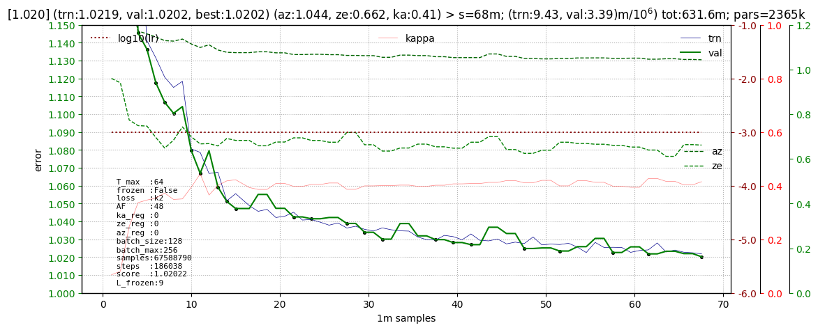
Let's show a typical training start schedule (pulses are DOM-aggregated). An error of the order of 1.020 when learning from scratch is achieved in 60-70 million examples (300 batches, not necessarily new ones). The total time on the standard T4 card is about 12 hours. This stage was done at a constant learning rate lr=1e-3 with the Adam optimizer:
It took significantly longer to get close to error 1.002. To achieve it, the learning rate was gradually decreased to 1e-5 (below, the dotted brown line). At the level of 1.004, there was a transition to large maxima of the sequence lengths. This immediately reduced the error by 1-1.5 points (see below, the DOM256 mark):
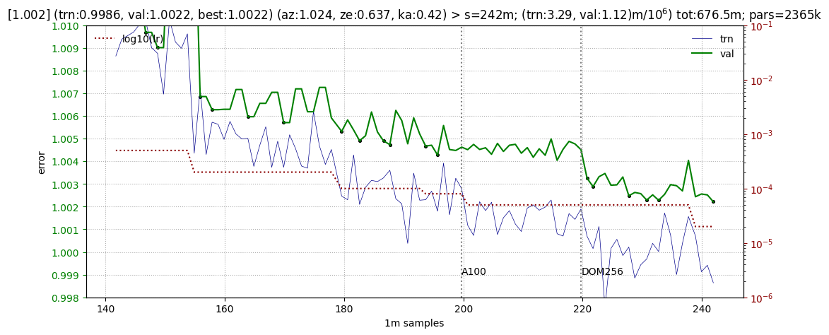
Further training required a transition to non-DOM-aggregated pulses and took a few more days on the A100 card.
During the training process, we analyzed the value of the weights on various blocks of the model and gradient propagation through them. A typical analysis chart looked like this:
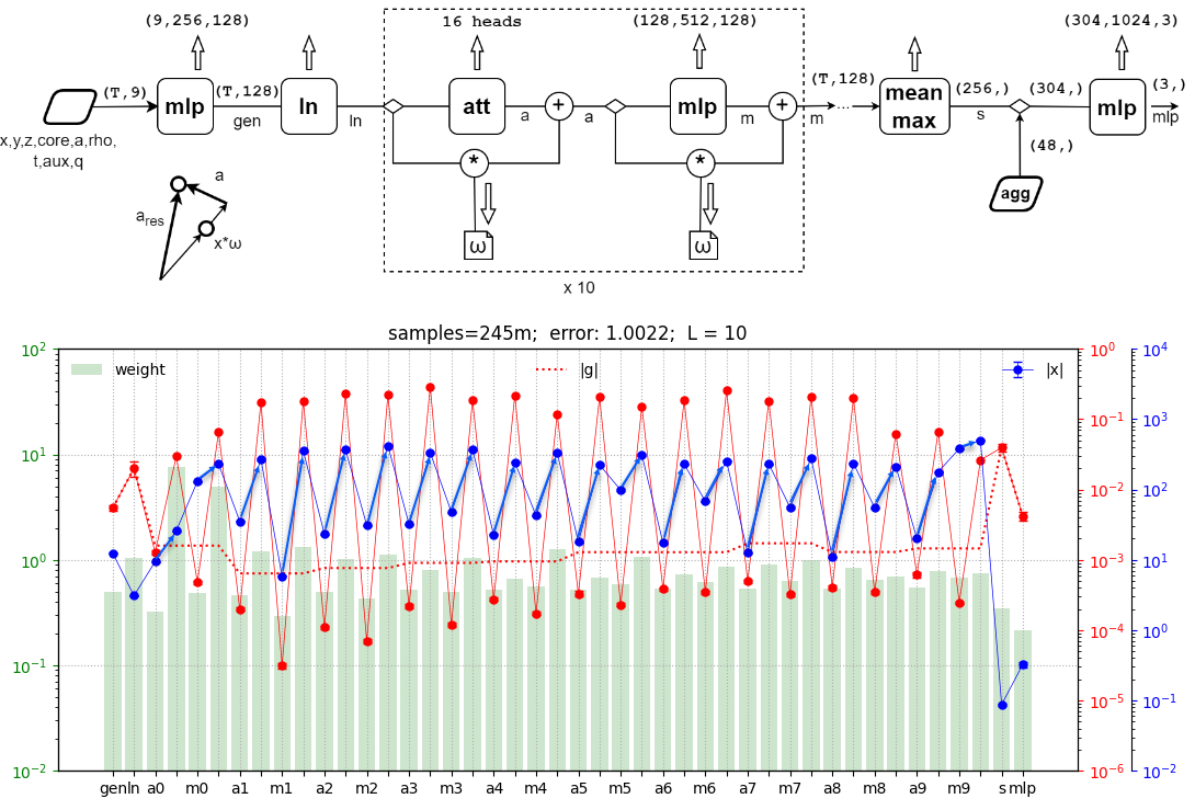
Vertical green bars are the average value of the parameter module on a particular network block. The red line is the value of the gradient on them and the blue line is the average value of the tensor components passing through the modulus.
This analysis was used to increase the number of transformer blocks on the already trained model. In addition, if some blocks "dropped out" according to their characteristics, we trained them separately, freezing the rest. Freezing the entire transformer was also used to retrain the final blocks of the model. Note that only requires_grad_(False) is not enough for this. It is necessary to block the construction of the computational graph, otherwise there will be no memory gain.
An analysis was also made of the influence of individual features and blocks of the model on the resulting metric. The structure of model errors was analyzed, depending on the various characteristics of the event (see for example). This analysis allowed to choose a more optimal model architecture.
What have not been done
- Use a bidirectional recurrent layer as integrator.
- Use the transformer pre-trained on the regression task to detect noise pulses, for their subsequent filtering.
- Replace the regressor with a classifier, for a large set of directions (points on a sphere). A similar model got to error 1.012, but there was not enough time to retrain it and include it in the ensemble.
- Train a model on a subset of the data (for example, single-string events, two-string events, etc.) by obtaining a set of models that specialize in specific event patterns.
- Add position embedding.