Simple reconstruction models
During this competition, in addition to machine learning methods, we also studied several "physical" methods of particle track reconstruction. Many of them are faster than machine learning models, although they mostly have lower accuracy. Below we present some formulas and programming code for this class of models.
Line-fit method
 Let the charge move along the trajectory \(\mathbf{r}=\mathbf{q} + \mathbf{u}\,t\)
and \(N\) sensors are triggered in the vicinity of the trajectory \(\{(t_i,\mathbf{r}_i)\},~i=1...N\).
We will minimize their distances \(D\) from the charge trajectory, that is:
$$
L = \bigr\langle D^2/\text{c}^2_\theta\bigr\rangle = \bigr\langle\bigr( \mathbf{q} + \mathbf{u}\,t - \mathbf{r }\bigr)^2\bigr\rangle = \min.
$$
Averaging (angle brackets) can be done with the weights \(w_i\):
$$
\langle f\rangle = \sum^N_{i=1} w_i\,f_i,~~~~~~~~~~~~~\sum^{N}_{i=1} w_i = 1.
$$
The gradients from the functional \(L\) at the minimum point are equal to zero:
$$
\frac{1}{2}\,\frac{\partial L}{\partial \mathbf{q}} = \mathbf{q} + \mathbf{u}\,\langle t \rangle - \langle \mathbf{r} \rangle = 0.
~~~~~~~~~~~~~~~~~
\frac{1}{2}\,\frac{\partial L}{\partial \mathbf{u}} = \mathbf{q}\,\langle t \rangle + \mathbf{u}\,\langle t^2 \rangle - \langle \mathbf{r} t \rangle = 0,
$$
This system of equations has the following solution:
$$
\mathbf{u} = \frac{\langle\mathbf{r}\,t\rangle - \langle\mathbf{r}\rangle\,\langle t\rangle}{\langle t^2\rangle - \langle t\rangle^2},~~~~~~~~~~~~~~~~~\mathbf{q} = \langle\mathbf{r}\rangle - \mathbf{u}\,\langle t\rangle.
$$
Let the charge move along the trajectory \(\mathbf{r}=\mathbf{q} + \mathbf{u}\,t\)
and \(N\) sensors are triggered in the vicinity of the trajectory \(\{(t_i,\mathbf{r}_i)\},~i=1...N\).
We will minimize their distances \(D\) from the charge trajectory, that is:
$$
L = \bigr\langle D^2/\text{c}^2_\theta\bigr\rangle = \bigr\langle\bigr( \mathbf{q} + \mathbf{u}\,t - \mathbf{r }\bigr)^2\bigr\rangle = \min.
$$
Averaging (angle brackets) can be done with the weights \(w_i\):
$$
\langle f\rangle = \sum^N_{i=1} w_i\,f_i,~~~~~~~~~~~~~\sum^{N}_{i=1} w_i = 1.
$$
The gradients from the functional \(L\) at the minimum point are equal to zero:
$$
\frac{1}{2}\,\frac{\partial L}{\partial \mathbf{q}} = \mathbf{q} + \mathbf{u}\,\langle t \rangle - \langle \mathbf{r} \rangle = 0.
~~~~~~~~~~~~~~~~~
\frac{1}{2}\,\frac{\partial L}{\partial \mathbf{u}} = \mathbf{q}\,\langle t \rangle + \mathbf{u}\,\langle t^2 \rangle - \langle \mathbf{r} t \rangle = 0,
$$
This system of equations has the following solution:
$$
\mathbf{u} = \frac{\langle\mathbf{r}\,t\rangle - \langle\mathbf{r}\rangle\,\langle t\rangle}{\langle t^2\rangle - \langle t\rangle^2},~~~~~~~~~~~~~~~~~\mathbf{q} = \langle\mathbf{r}\rangle - \mathbf{u}\,\langle t\rangle.
$$
The length of the vector \(\|\mathbf{u}\|\), calculated by these formulas, can generally turn out to be not unity (i.e. the speed of light). Note that the speed \(\mathbf{u}\) does not change when the time point of reference is shifted \(t\mapsto t-t_0\). In this case, the position vector of the trajectory changes: \(\mathbf{q}~=~ \langle\mathbf{r}\rangle - \mathbf{u}\,\langle t-t_0\rangle\). By choosing \(t_0\) one can, for example, achieve orthogonality of \(\mathbf{q}\) and \(\mathbf{u}\). Further, we assume that \(|\mathbf{u}|=c=1\) (in the natural system of units): $$ \mathbf{q} = \langle\mathbf{r}\rangle - \langle \mathbf{r}\mathbf{u} \rangle\,\mathbf{u},~~~~~~~~~~t_0=\langle t \rangle - \langle \mathbf{r}\mathbf{u} \rangle,~~~~~~~~~~~\mathbf{u}^2=1,~~~~~\mathbf{q}\mathbf{u}=0. $$
Python implementation
The following is an example of programmatic implementation of the line-fit method using the pandas library:
def line_fit(df, lm = 5.5, eps = 1e-8):
    """ Weighted Line-fit method """
    df['w']   = np.exp(-lm * df.t)

    df['xw']  = df.x * df.w;     df['yw']  = df.y*df.w;       df['zw']  = df.z*df.w;
    df['xtw'] = df.x*df.t*df.w;  df['ytw'] = df.y*df.t*df.w;  df['ztw'] = df.z*df.t*df.w;
    df['ttw'] = df.t*df.t*df.w;  df['tw']  = df.t*df.w;
    agg = df.groupby(["event_id"]).agg(
        xw  = ('xw', 'sum'), yw  = ('yw', 'sum'), zw  = ('zw', 'sum'), tw = ('tw', 'sum'),
        xtw = ('xtw','sum'), ytw = ('ytw','sum'), ztw = ('ztw','sum'), ttw= ('ttw','sum'),
        w   = ('w',  'sum')
    )
    agg.xw  /= agg.w;  agg.yw  /= agg.w; agg.zw  /= agg.w;  agg.tw  /= agg.w;
    agg.xtw /= agg.w;  agg.ytw /= agg.w; agg.ztw /= agg.w;  agg.ttw /= agg.w;

    agg['Dtw'] = agg.ttw - agg.tw*agg.tw
    agg['ux'] = ( agg.xtw - agg.xw*agg.tw ) / ( agg.Dtw + eps);
    agg['uy'] = ( agg.ytw - agg.yw*agg.tw ) / ( agg.Dtw + eps);
    agg['uz'] = ( agg.ztw - agg.zw*agg.tw ) / ( agg.Dtw + eps);

    agg['qx'] = agg.xw - agg.ux * agg.tw
    agg['qy'] = agg.yw - agg.uy * agg.tw
    agg['qz'] = agg.zw - agg.uz * agg.tw
    return agg[['ux', 'uy', 'uz', 'qx', 'qy', 'qz' ]]
Note that GPU calculations using the pytorch library can significantly speed up the above calculations.
We found that using weights that decrease for the later-in-time pulses significantly improves the metric. For the lm ~ 5 parameter, the angular error is 1.180:
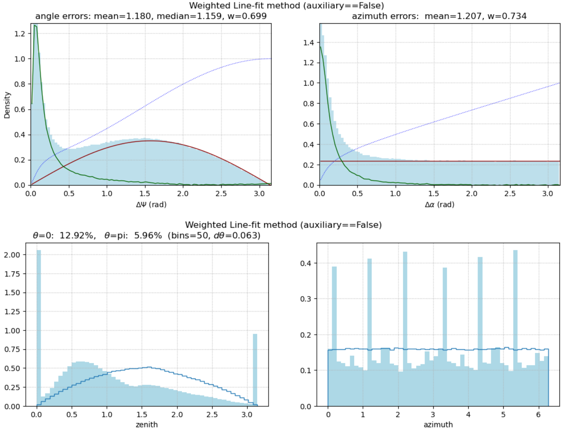
With equal weights for all pulses, the error is 1.220. It's worth mentioning that the line-fit method is very sensitive to pulse quality and only works if auxiliary=False.
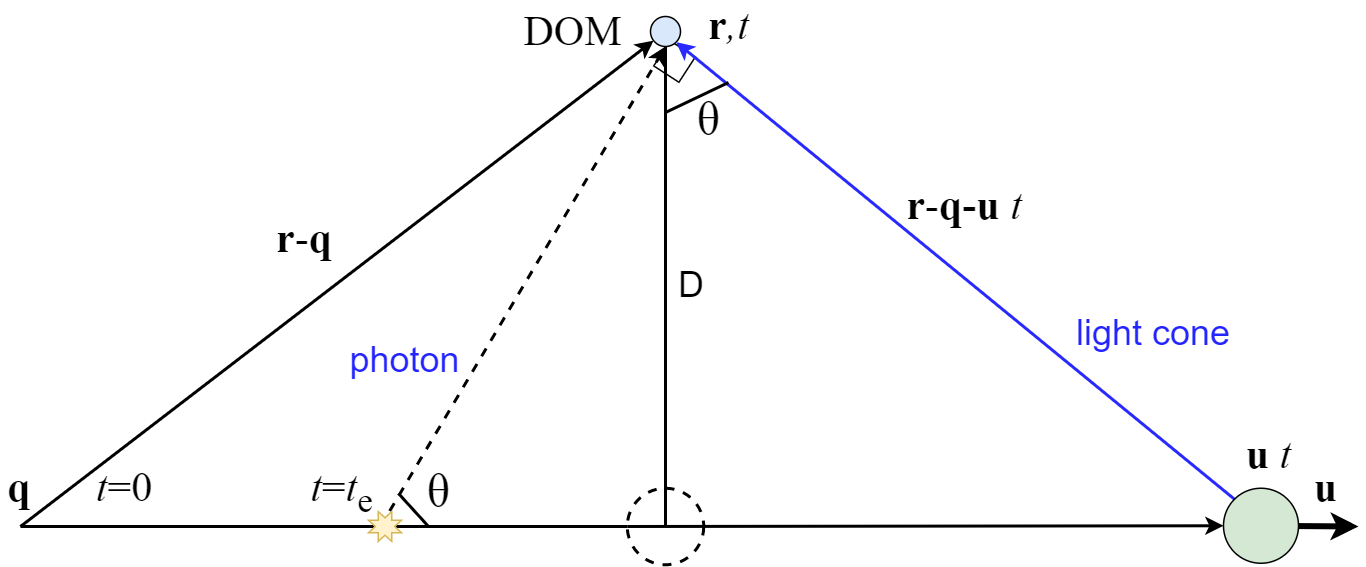
Method Santa
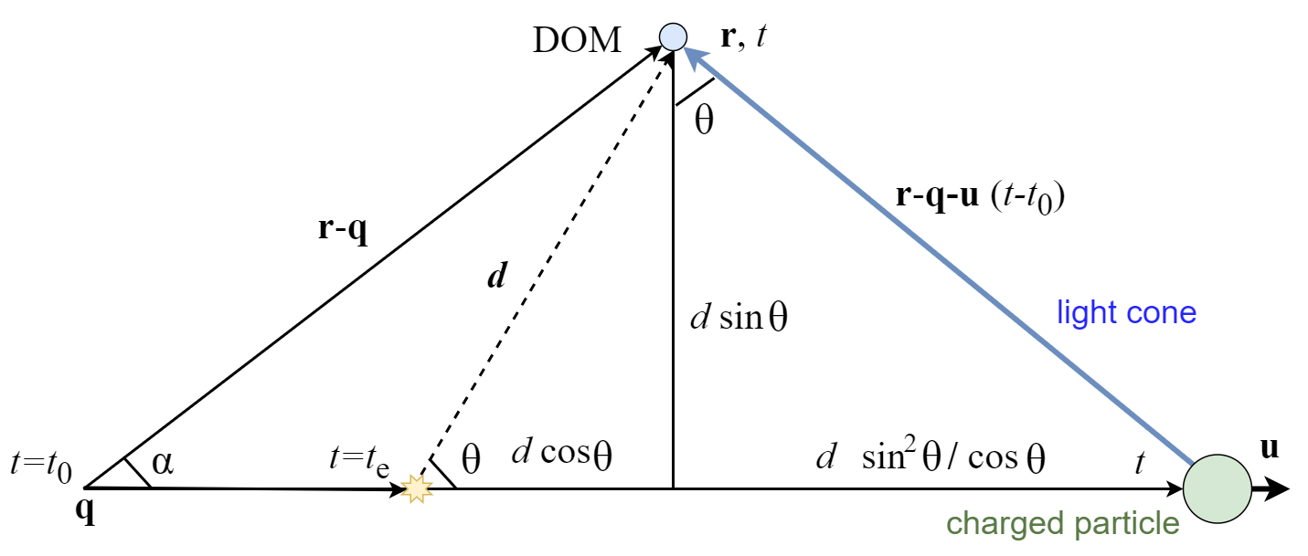
The light cone of Cherenkov radiation has an angle \(\cos\theta = 1/n\) (again, we use \(|\mathbf{u}|=c=1\)). Let's write the length of the line from DOM going at a perpendicular to the path as a common side of two right triangles: $$ d\,\sin\theta = \|\mathbf{r}-\mathbf{q}\|\,\sin\alpha $$ A charge with a speed \(u=1\) travels over the time \(t\) the distance: $$ t-t_0 = (\mathbf{r}-\mathbf{q})\,\mathbf{u} + d\,\frac{\sin^2\theta}{\cos\theta}. $$ Substituting \(d\) and given that \(\|(\mathbf{r}-\mathbf{q})\times\mathbf{u}\| = \|\mathbf{r}-\mathbf{q}\|\,\sin\alpha = \sqrt{(\mathbf{r}-\mathbf{q})^2 - ((\mathbf{r}-\mathbf{q})\cdot\mathbf{u})^2}\), we get: $$ t-t_0 = (\mathbf{r}-\mathbf{q})\,\mathbf{u} + \mu\,\|(\mathbf{r}-\mathbf{q})\times\mathbf{u}\|,~~~~~~~~~~~~\mu =\tan\theta. $$ If we choose the origin \(t=t_0\) for which the vectors \(\mathbf{u}\) and \(\mathbf{q}\) are orthogonal, then: $$ t-t_0 = \mathbf{r}\mathbf{u} + \mu\,\sqrt{(\mathbf{r}-\mathbf{q})^2 - (\mathbf{r}\mathbf{u})^2 },~~~~~~~~~~\mathbf{u}^2=1,~~~~~~~\mathbf{q}\mathbf{u}=0. $$ In the Santa method, the deviations of the sensor response times from this theoretical expression are minimized under the constraints \(\mathbf{u}^2=1\), \(\mathbf{q}\cdot\mathbf{u}=0\): $$ \left\langle\Bigr(~t -t_0 - \mathbf{r}\,\mathbf{u} - \mu\,\sqrt{(\mathbf{r}-\mathbf{q})^2 - (\mathbf{r}\mathbf{u})^2 } ~\Bigr)^2\right\rangle = \min. $$ In particular, for given (orthogonal) \(\mathbf{u}\), \(\mathbf{q}\) it is easy to find the optimal \(t_0\): $$ t_0 ~=~ \left\langle~t - \mathbf{r}\mathbf{u} - \mu\,\sqrt{(\mathbf{r}-\mathbf{q})^2 - (\mathbf{r}\mathbf{u})^2 } \right\rangle . $$ Knowing it, one can find the times that deviate greatly from theoretical values. Especially big deviations are \(t_i \lt t\), since the sensor could not fire before the cone.
Python implementation
When solving the Santa minimization problem by the gradient (or simplex) method, these 5 parameters can be used: \((t_0,\,\alpha,\,\beta,\,\gamma,\,q)\), in terms of which: $$ \mathbf{u}=\{~\text{s}_\beta\,\text{c}_\alpha,~\text{s}_\beta\,\text{s}_\alpha,~\text{c}_\beta~\},~~~~~~~~~ \mathbf{q}~=~q~ \{~\text{c}_\gamma u_z,~\text{s}_\gamma u_z,~-\text{c}_\gamma u_x-\text{s}_\gamma u_y~\} =q~ \{~\text{c}_\gamma \,\text{c}_\beta,~\text{s}_\gamma \,\text{c}_\beta,~-\text{c}_{\gamma-\alpha}\,\text{s}_\beta ~\}, $$ where \(\text{s}_\beta = \sin\beta\) and so on.
It was planned to minimize the functional on the GPU in batch mode. This should significantly speed up the calculation of track parameters. However, we have not yet begun this task. :)