Loss functions
Neutrino trajectory reconstruction can be solved as a regression or classification problem. In the latter case, the directions (points on the unit sphere) are divided into classes; then, the standard error of cross-entropy is applied. In the regression approach to the problem, the choice of the error function is much wider. Below some options are described.
Predicting directly the azimuth and zenith angles is not feasible, due to their ambiguity (periodicity). Therefore, the model predicts three components of the direction vector \(\hat{\mathbf{n}}\), which is not necessarily a unit vector. At the same time, the target vector \(\mathbf{n}\) is indeed a unit one \(\mathbf{n}^2=1\). Our task is to minimize the angle between the vectors: $$ \cos\Psi = \frac{\mathbf{n}\hat{\mathbf{n}}}{\|\hat{\mathbf{n}}\|},~~~~~~~~~\text{error} = \langle\Psi\rangle ~\in~ [0...\pi] = \min. $$
At first glance, it seems reasonable to minimize the competition metric \(\Psi\) directly: $$ \mathcal{L}_0(\mathbf{n},\hat{\mathbf{n}}) ~=~ \Psi ~=~\arccos \frac{\mathbf{n}\hat{\mathbf{n}}}{\|\hat{\mathbf{n}}\|} $$ However, this metric has a singular gradient value, which can lead to unstable learning. When constructing a computational graph, the gradient from \(\arccos \) will first be obtained: $$ (\arccos x)' = -\frac{1}{\sqrt{1-x^2}} = -\frac{1}{\sin\Psi}. $$ Analytically, the sine in the denominator will cancel out, but numerically there is a high probability of getting a division by zero (NaN).
The next natural choice is MSE error equal to the distance between the two vectors: $$ \mathcal{L}_1(\mathbf{n},\hat{\mathbf{n}}) = (\mathbf{n}-\hat{\mathbf{n}})^2 = (n_x-\hat{n}_x)^2+(n_y-\hat{n}_y)^2+(n_z-\hat{n}_z)^2 $$ The MSE gradient is "almost perfect". However, this error does not care much about the direction: for \(\Psi\sim 0\) and large \(\|\hat{\mathbf{n}}\|\) the error can be larger than for \(\Psi = \pi\), but \(\|\hat{\mathbf{n}}\|\sim 0\). In our problem, there are many noisy events with large errors between the target and the predicted vector. Therefore, we did not use MSE errors.
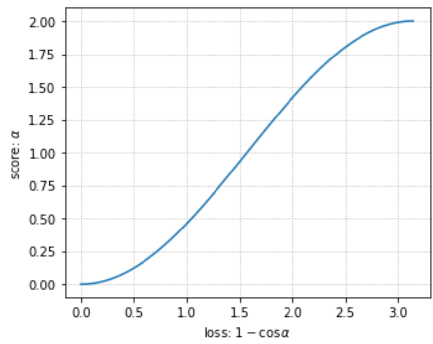 More optimal is Cosine Loss:
$$
\mathcal{L}_2(\mathbf{n},\hat{\mathbf{n}}) = 1-\cos(\Psi)= 1-(\mathbf{n}\hat{\mathbf{n}})/\|\hat{\mathbf{n}}\|
$$
However, for small lengths \(\|\hat{\mathbf{n}}\|\) computational problems may arise, as
$$
\left(\frac{\partial \mathcal{L}_2}{\partial \hat{\mathbf{n}}}\right)^2
= \frac{\sin^2\Psi}{\|\hat{\mathbf{n}}\|^2}
$$
Therefore, the gradient decays at large lengths \(\|\hat{\mathbf{n}}\|\) and explodes at \(\|\hat{\mathbf{n}}\|\sim 0\)
(and we have no control over the value of \(\|\hat{\mathbf{n}}\|\) ).
In addition, it vanishes at \(\Psi=0\) (this is normal), but also at \(\Psi=\pi\) (it is difficult to turn around the direction of prediction).
More optimal is Cosine Loss:
$$
\mathcal{L}_2(\mathbf{n},\hat{\mathbf{n}}) = 1-\cos(\Psi)= 1-(\mathbf{n}\hat{\mathbf{n}})/\|\hat{\mathbf{n}}\|
$$
However, for small lengths \(\|\hat{\mathbf{n}}\|\) computational problems may arise, as
$$
\left(\frac{\partial \mathcal{L}_2}{\partial \hat{\mathbf{n}}}\right)^2
= \frac{\sin^2\Psi}{\|\hat{\mathbf{n}}\|^2}
$$
Therefore, the gradient decays at large lengths \(\|\hat{\mathbf{n}}\|\) and explodes at \(\|\hat{\mathbf{n}}\|\sim 0\)
(and we have no control over the value of \(\|\hat{\mathbf{n}}\|\) ).
In addition, it vanishes at \(\Psi=0\) (this is normal), but also at \(\Psi=\pi\) (it is difficult to turn around the direction of prediction).
Scalar proximity is one more option, and it minimizes the scalar product as above. At the same time, the predicted vector \(\hat{\mathbf{n}}\) is not normalized, but we inhibit the larger values of its length: $$ \mathcal{L}_3(\mathbf{n},\hat{\mathbf{n}}) = -(\mathbf{n}\hat{\mathbf{n}}) + \lambda\,\hat{\mathbf{n}}^2 = -\|\hat{\mathbf{n}}\|\,\cos\Psi + \lambda\,\hat{\mathbf{n}}^2. $$ This error could go in two directions - increase the cosine to 1 or increase the length of the vector indefinitely. But the latter is suppressed due to the regularisation term.
For \(\lambda = 1/2\) the error derivative with respect to \( \|\hat{\mathbf{n}}\| \) is equal to \( -\cos\Psi + \|\hat{\mathbf{n} }\|\). In the optimal value \( \Psi=0 \) the minimum error will correspond to the unit vector. It is this error with the parameter \( \lambda = 1/2 \) that was mainly used when training the Transformer model.
von Mises-Fisher loss (vMF) is used in the GraphNet architecture. Our experiments have shown its usefulness for models with other architectures as well. Below is the content of our post on kaggle about adapting this error for the 3D case.
Explanation and Improvement of von Mises-Fisher Loss
Practical part
The vMF-loss maximizes the scalar product of the true and predicted vectors and adds a "regularization term" that depends on the length of the predicted vector: $$ \mathcal{L}(\hat{\mathbf{n}},\,\mathbf{n}) = - \hat{\mathbf{n}}\,\mathbf{n} +\log (2\pi) +\kappa - \log\kappa + \log \bigr(1-e^{-2\kappa} \bigr),~~~~~~~~~~~\kappa=\|\hat{\mathbf{n}}\|. $$
The implementation of this vMF-loss is very simple (omitting the constant \(2\pi\)):
def vMF_loss(n_pred, n_true, eps = 1e-8):
    """  von Mises-Fisher Loss: n_true is unit vector ! """
    kappa = torch.norm(n_pred, dim=1)
    logC  = -kappa + torch.log( ( kappa+eps )/( 1-torch.exp(-2*kappa)+2*eps ) )
    return -( (n_true*n_pred).sum(dim=1) + logC ).mean()
It is worth comparing it with the original implementation from GraphNet, given, for example, in this post.
First of all, they are numerically equivalent.
However, GraphNet uses the general vMF-loss for m-dimensional space.
In three-dimensional space, the modified Bessel functions are reduced to elementary functions.
In addition, there is no need to partition the range of variation \(\kappa\) and use an approximate
formula to eliminate the overflow.
This loss function is also well behaved at zero \(\kappa=0\), unlike the one used in GraphNet.
The empirical part
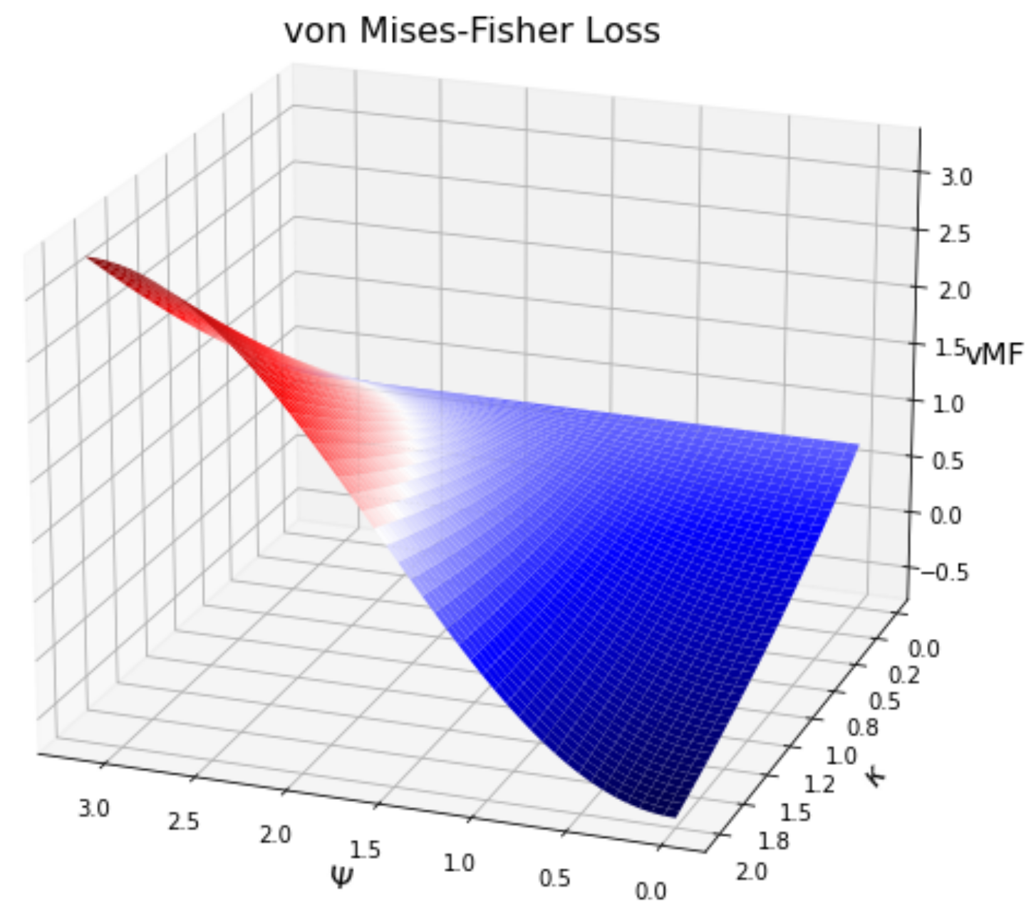 Before we dive into the math, let's understand the empirical meaning of the above expression.
Let's express the scalar product as a function of the error angle between the vectors \(\mathbf{n}\,\hat{\mathbf{n}}=\kappa\,\cos\Psi\)
and plot the loss as a function of the angle \(\Psi\) and the vector length \(\kappa\).
Before we dive into the math, let's understand the empirical meaning of the above expression.
Let's express the scalar product as a function of the error angle between the vectors \(\mathbf{n}\,\hat{\mathbf{n}}=\kappa\,\cos\Psi\)
and plot the loss as a function of the angle \(\Psi\) and the vector length \(\kappa\).
As can be seen, the loss decreases as the angle tends to zero with a simultaneous increase in \(\kappa\). For the gradient to reach the minimum, we don't need \(\kappa\) itself to grow, although in a notebook dedicated to GraphNet, large values of \(\kappa\) are used to select well-trained examples. However, the main thing is that the decrease in loss occurs in the direction of decreasing the error angle; and that's exactly what we need.
Theoretical part
Let's now give a mathematical justification to von Mises-Fisher Loss. Let the probability of deviation of a 3-dimensional unit vector \(\hat{\mathbf{n}}\) from a fixed unit vector \(\mathbf{n}\) be described by the von Mises-Fisher (vMF) distribution : $$ p(\hat{\mathbf{n}}| \mathbf{n}) = C(\kappa)\, e^{\kappa\, \hat{\mathbf{n}}\cdot\mathbf{n}} = C(\kappa)\, e^{\kappa\, \cos\Psi}. $$ If the vectors are the same: \(\hat{\mathbf{n}}\mathbf{n}=1\) - the probability is maximal; if they have the opposite direction, \(\hat{\mathbf{n}}\mathbf{n}=-1\) is minimal. The probability decay rate is characterized by the \(\kappa\) (concentration parameter). The value of \(\kappa=0\) defines a uniform distribution over the hypersphere and \(\kappa = \infty\) defines a point distribution at \(\mathbf{n}\). If the angle \(\Psi\) between the vectors \(\hat{\mathbf{n}}\) and \(\mathbf{n}\) is small, then we simply get a normal distribution: \(p(\hat{\mathbf{ n}}| \mathbf{n}) \sim e^{-\kappa\, \Psi^2/2}\).
To find the normalization constant \(C\) of the distribution, it is necessary to calculate the integral over the entire space \(\hat{\mathbf{n}}\). Since this vector is a unit vector, in three-dimensional space it is easy to do this in a spherical coordinate system by choosing the \(z\) axis along the vector \(\mathbf{n}\). Simple integration gives: $$ \int\limits^{2\pi}_0 d\phi \int\limits^\pi_0 \sin\Psi \, d\Psi\,\, C\, e^{\kappa \cos\Psi} = 2\pi\,C\, \int\limits^1_{-1} dz\,\, e^{\kappa z} = \frac{2\pi\,C}{\kappa}\,\Bigr(e^{\kappa}-e^{-\kappa}\Bigr) = 1. $$ In an m-dimensional space, the result of such an integration would not be possible to express in elementary functions. In three-dimensional space, we get the simple expression: $$ C(\kappa) = \frac{1}{2\pi}\,\frac{\kappa\,e^{-\kappa}}{1-e^{-2\kappa} }. $$ Note that the normalization factor is finite at zero: \(C(0)=1/4\pi\).
Let the model output vector \(\hat{\mathbf{n}}\), as well as the target vector \(\mathbf{n}\) be normalized to one. We will maximize the probability \(p(\hat{\mathbf{n}}| \mathbf{n})\), or, equivalently, minimize its negative logarithm (log-likelihood): $$ \mathcal{L}(\hat{\mathbf{n}},\,\mathbf{n}) = -\log p(\hat{\mathbf{n}}| \mathbf{n}) = -\kappa\,(\hat{\mathbf{n}}\cdot\mathbf{n}) - \log C(\kappa). $$ At this point, it is necessary to move away from mathematics and turn to magic. Above, we considered that \(\kappa\) is a constant characterizing the sharpness of the probability distribution. Let us now assume that this is not a constant, but the length of the predicted vector \(\kappa=\|\hat{\mathbf{n}}\|\) before its normalization. As a result, the distribution will be close to uniform (the loss is large) for small lengths \(\hat{\mathbf{n}}\). For large \(\kappa\), the loss will be smaller. Now we can consider that the vector \(\hat{\mathbf{n}}\) is not actually normalized, assuming that \(\kappa\,(\hat{\mathbf{n}}\cdot\mathbf{n}) \mapsto \hat{\mathbf{n}}\cdot\mathbf{n}\) and \(\hat{\mathbf{n}}\) has an arbitrary length equal to \(\kappa\).
How many bad samples there are in the dataset?
Let's investigate how the prediction error is related to the characteristics of neutrino events.
Our models predict not angles but rather the direction vector. This vector is compared with the target vector.
The angle \(𝛥ψ\) between them is the model error (angular error).
Another angle (azimuthal error \(𝛥α)\) is calculated between the projections of the target and predicted vectors onto the \((x,y)\) plane.
Zenith angle errors did not yet give us any interesting information.
For the \(𝛥ψ\) and \(𝛥α\) angles, the histograms are plotted, given below by three algorithms:
Weighted Line-fit method, RNN and GNN:
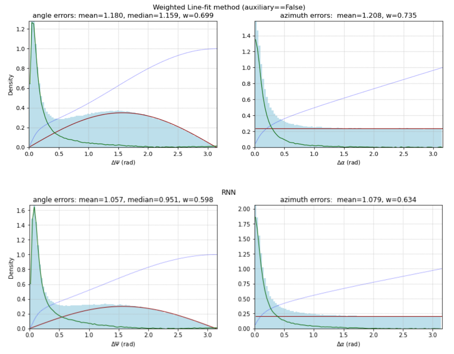
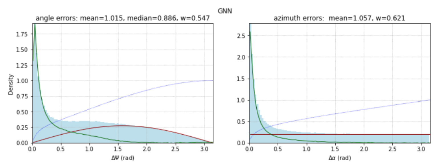
The average angular error is the metric for our competition. In addition to the mean, we calculate the median, which is usually used in physical publications when comparing different methods of trajectory reconstruction. In all our models, the median is lower than the mean (and the better the model, the greater this difference).
In addition to these two characteristics, we evaluate the proportion of examples that turned out to be “bad” (that is, not predicted accurately) for a given method.
Let’s assume that all examples for angular errors can be divided into two classes - “good” and “bad”. The proportion of bad examples is \(w\), and of good examples, \(1-w\). Then the distribution of errors of both classes has the form:
$$ P(ψ) = (1-w) P_0(ψ) + w \, \sin(ψ) / 2 $$The second term is the distribution of the angle \(ψ = [0, π]\) between a fixed (target) vector and a vector with a random isotropic direction. For more or less working prediction methods, the first term \(P_0(ψ)\) decreases rapidly. Therefore, to estimate the weight \(w\), the distribution integral is used in the range \([π/2, π]\) in which the distribution of random errors predominates. The calculated values of this weight are given above in the headings of the histograms. Knowing \(w\), we can construct the error distribution of “good examples” (green line) and “bad” ones (red line). The dotted line is the cumulative probability distribution from the cumulative histogram.
In the case of azimuth errors, the cumulative distribution is approximated as follows:
$$ P(α) = (1-w) P_0(α) + w / π, $$The distribution of “bad events” in this case is a uniform distribution.
As can be seen from the figures above, the proportion of “bad events” by different methods gives close enough results: 60% - 70%. Although as the method improves, this value gradually decreases. :) Note that when calculating the projections of vectors on the plane \((x, y)\), it is necessary to control for their length in this plane. If the length turns out to be equal to zero, the angle should be chosen randomly from the uniform distribution \([0…π]\). If this is not done, a sharp outlier will be observed on the distribution in the Line-fit method at \(α=π/2\). It corresponds to single string events in which the sensors are triggered on only one string. In the dataset, with the auxiliary==False filter (only “reliable” pulses), there are 17.7% of single-string events:
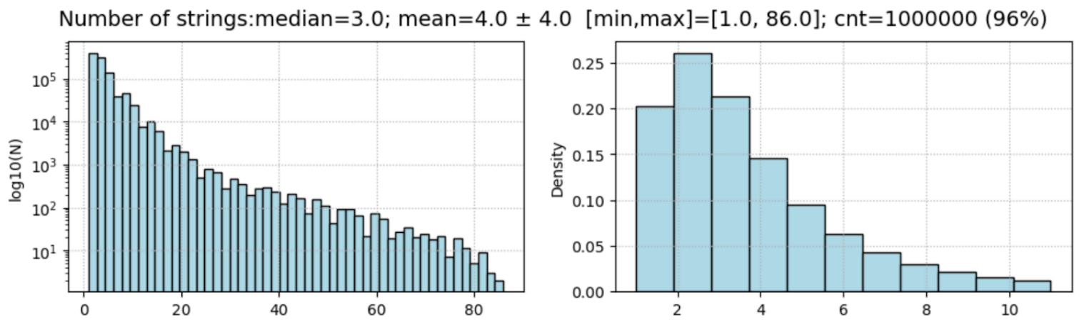
Clearly, for single-string events, Line-fit predicts the direction vector along the string. Therefore, its projection on the plane \((x,y)\) will be equal to zero, and the value of the azimuth angle is not defined.
The distributions of the predicted zenith and azimuth angles also look quite interesting:
Two large values for bins at the zenith angles 0 and π are associated with single-string events (17.7%). On the rest of the distribution, one can also distinguish a random part of sin/2 and a “non-random” one. The six peaks in the distribution of azimuthal angles are related to the “discrete hexagonality” of space in the \((x,y)\) plane.
The implementation of the function that builds the error distribution for the Line-fit method can be found in the notebook. We use weighted averages, which results in reducing the error from 1.21 to 1.18.