GNN model
Our model "GNN" is a modification of the graph neural network architecture for Neutrino Telescope Event Reconstruction, which is described in detail in the paper Graph Neural Networks for Low-Energy Event Classification & Reconstruction in IceCube and available on github: GraphNet.
The overall structure of the architecture is as follows:
- \(x,y,z\) - coordinates;
- \(t\) - time;
- \(q\) - charge;
- \(aux\) - auxilary
- \(homophily(x,y,z,t)\) - similarity of features in graph nodes;
- \(mean(x,y,z,t,q,aux)\) - mean values of pulse features;
- \(pulses\) - number of pulses in an event;
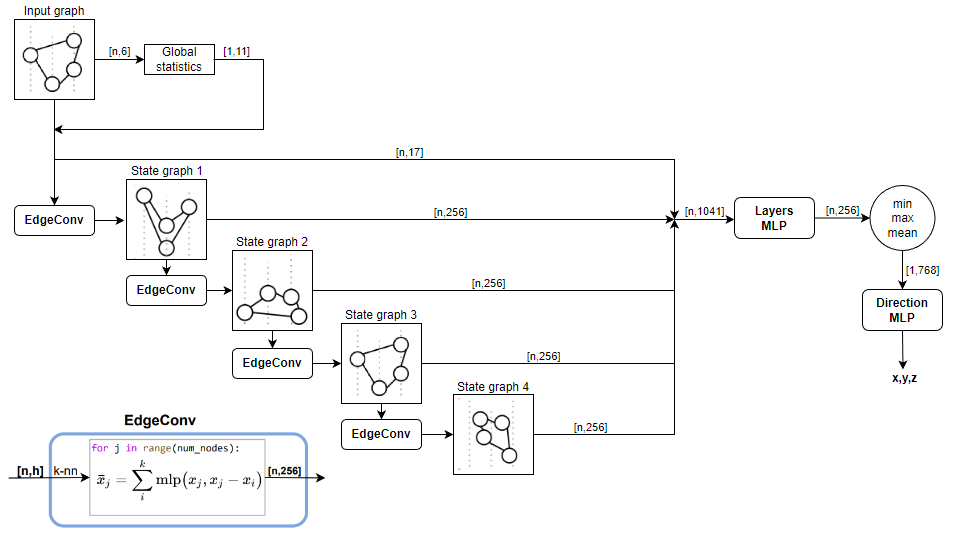
Thus, for each event, we get a graph in which each node corresponds to the pulse, and the features are the features of the pulse combined with the aggregated features of the event.
The resulting graph sequentially passes through layers, each of which modifies the feature space and also updates its topology. The outputs of all layers are combined and fed to the layer Layers MLP in which the number of features is reduced to 256. Then a pooling operation is performed in which the features of all nodes of the graph are aggregated by functions min, max, mean. Accordingly, we obtain 768 features for each event.
Since the purpose of the architecture is to predict the direction, at the last nodeDirection MLP the resulting embedding is converted into a 3D direction vector.
Training and enchancing the model
Training base model (1.018 → 1.012)
Since we were limited in computational resources, we decided to proceed with retraining the best public GNN model from a notebook GraphNeT Baseline Submission (special thanks to @rasmusrse) which gave LB score 1.018. Using the library polars we accelerated the batch preparation time to 2 seconds. We retrained the model on all batches, except for the last one; 100k examples of batche 659 were used for validation. An epoch corresponded to one batch (200k events); minibatch size: 400 events. So, in each epoch:- the previous batch was unloaded from memory;
- new one loaded in 2 seconds;
- training was done for 500 (200k/400) steps in 1-2 minutes depending on the architecture and the freezing of the layers;
- validation was performed in 20 seconds;
- model weights were saved if the loss function or metric reached a new minimum;
Here, special thanks are due to Google Colab Pro, without which we would not have been able to train such an architecture within reasonable timeframe.
As a result, after 956 epochs, the value of the metric dropped to 1.0127.
Adding another layer (1.012 → 1.007)
Having a trained network, we tried to add another layer EdgeConv to it. In order not to learn from scratch, all layers in the new architecture were frozen except for the new one.In the frozen layers, weights were loaded from the model retrained at the previous stage and training continued.
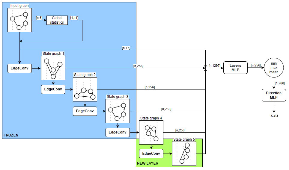
After 1077 epochs, we reached the metric 1.007
Increasing the number of neighbors (1.007 → 1.003)
In the original Graphnet library, the number of neighbors for building a graph is chosen as 8.We have tried increasing this value to 16
Thus, we retrained the trained model from the previous stage with a new number of neighbors.
After the 1444 epochs, the metric reached a new low of 1.003
Expanding Layers MLP(1.003 → 0.9964)
Since the number of layers was increased, we thought it reasonable that the number of parameters of Layers MLP which receives concatenated input of the outputs of each level, should also be increased. The first layer of the module Layers MLP was increased from 336 to 2048. Similarly, all levels were frozen, the weights of the model of the previous stage were loaded, and training was continued.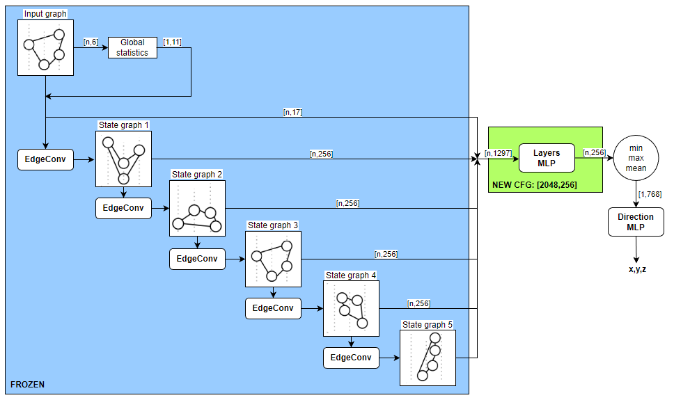
After 1150 epochs, the metric dropped to 0.9964
Replacing regression with classification (0.9964 → 0.9919)
Studying the best solutions, we paid attention to the notebook Tensorflow LSTM Model Training TPU (thanks to @rsmits) From it we borrowed the idea to move from a regression problem to a classification one.The azimuth angle was uniformly divided into 24 bins.
azimuth_edges = np.linspace(0, 2 * np.pi, bin_num + 1)
The zenith angle was also divided into 24 bins; here we warked with cosine of zenith, since it is the cosine that has a uniform distribution (as is seen from the statistics of all training events):
for bin_idx in range(1, bin_num):
    zenith_edges.append(np.arccos(np.cos(zenith_edges[-1]) - 2 / (bin_num)))
Accordingly we received a total of 24x24=576 classes.
The the last layer of MLP was increased from [128,3] to [512,576], and the loss-function was changed to CrossEntropyLoss.
We froze the entire model except for the last module.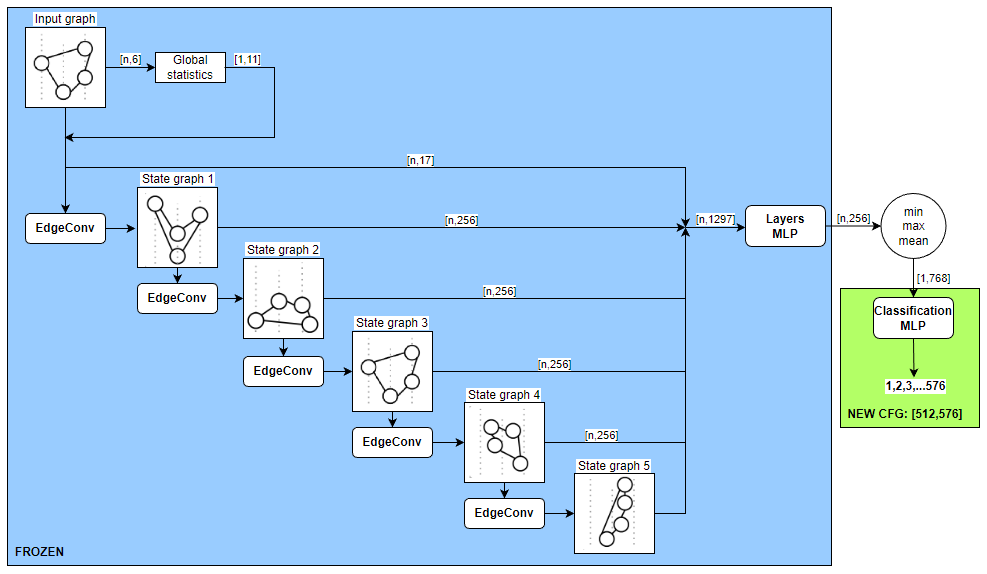
After 967 epochs, the metric reached the value of 0.9919.
This was the best result that we achieved for a standalone GNN model, and it was then used for ensembling with other models.
What didn't help
During the competition we tried many other things that did not yield a noticeable improvement of the metric, or none at all. Some of the things we did:
- separately predicting zenith and azimuth angles;
- changing the type of convolution to SAGE, GAT;
- inserting transformer after Layers MLP;
- replacing pooling with RNN (GRU);
- inserting a TopKPooling layer;
- using 4 or more features to build the event graph.
What have not been done
There are also several approaches which we thought over but did not pursued to the end, mainly because of lack of time and hardware resources, to mention just a few:
- training the GNN from scratch, with scattering, absorption and DOM-embedding features;
- training a classifier with a larger number of bins;
- parallel training of transformer and GNN models.